For more information contains additional functionality, configuration details, and summarized information. You can also refer to the Software Index to review specific topics.
For more information : Software Key Features
Key Features
Open software for high flexibility and multiple choices of testing Parameters can be adjusted (force, speed, …) can be monitored and changed during testing
Programming step-per-step Multiple choices of parameters in one single programEasy duplication of multiple steps: parameters of one step of programming can be copied and paste
Programmable servo-control of lower motion stages, including speed, direction, acceleration/deceleration rate, distance, angular position.
Multiple recipes savedPrograms for each user can be saved
Positioning controlPosition for the testing (X,Y,Z) can be programmed in the software
No time limit for the test acquisition
Real time data display.
Test protocols per several ASTM/DIN/ISO standards for automated execution.ASTM G77, G99, G119, G132, G133, G174, G176, D5183, DIN 50324, DIN 51834, …
Software application for post-test data analysis and report generation
Programmable test procedures, including test time, load, speed, frequency, distance, number of cycles, etc.
Automatic stribeck curve generation and data analysis.
Programmable test interruption upon meeting pre-set criteria (Friction, COF, distance, wear, AE, temperature, etc.),
Sample stage automated repositioning for surface inspection, test continuation .
Programmable control of environmental chambers.
Additional sensors (position, distance, temperature, resistance, etc.) data recording and display.Up to 16 additional channels
3 set of adjustable PID (for load, temperature, speed, …)
Same software for Tribology, Scratch, Indentation, Microscopy, … to allow combine testing.
Loop/delay functionality
For 3D imaging, 3D, profile and roughness, wear volume analysis included in MFT
All our file are save text with “.csv” or .”bin” extension. (Easy compatibility with Excel or Origin)
Start the software
Initialization window
Initialization window
When launching Rtec MFT software, the status window automatically opens. This window shows the initialization of all the machine components.
Status Window successfully initialized (Left), unsuccessful (Right)
If any issue appeared during initialization, it will appear as a red line. On the image, the red line shows that the initialization of the scratch module was not successful.
Initialization should be successful for the software to work properly. If it’s not, please restart the computer. If the error persists, contact customer service.
Software Key Features
Key Features
Open software for high flexibility and multiple choices of testing Parameters can be adjusted (force, speed, …) can be monitored and changed during testing
Programming step-per-step Multiple choices of parameters in one single programEasy duplication of multiple steps: parameters of one step of programming can be copied and paste
Programmable servo-control of lower motion stages, including speed, direction, acceleration/deceleration rate, distance, angular position.
Multiple recipes savedPrograms for each user can be saved
Positioning controlPosition for the testing (X,Y,Z) can be programmed in the software
No time limit for the test acquisition
Real time data display.
Test protocols per several ASTM/DIN/ISO standards for automated execution.ASTM G77, G99, G119, G132, G133, G174, G176, D5183, DIN 50324, DIN 51834, …
Software application for post-test data analysis and report generation
Programmable test procedures, including test time, load, speed, frequency, distance, number of cycles, etc.
Automatic stribeck curve generation and data analysis.
Programmable test interruption upon meeting pre-set criteria (Friction, COF, distance, wear, AE, temperature, etc.),
Sample stage automated repositioning for surface inspection, test continuation .
Programmable control of environmental chambers.
Additional sensors (position, distance, temperature, resistance, etc.) data recording and display.Up to 16 additional channels
3 set of adjustable PID (for load, temperature, speed, …)
Same software for Tribology, Scratch, Indentation, Microscopy, … to allow combine testing.
Loop/delay functionality
For 3D imaging, 3D, profile and roughness, wear volume analysis included in MFT
All our file are save text with “.csv” or .”bin” extension. (Easy compatibility with Excel or Origin)
Start the computer.
On the Dekstop, Click On the Rtec MFT Software.
Wait for the softwares to initialize.
For proper initialization of the machine, it is recommended to turn on the machine first, wait 30 seconds and then turn on the software.
Ensure that the tester’s switchs are On
Switching On the MFT-5000
The two AC Switches on the back of the machine, and the front ARU Button is disengaged.
Switching On the MFT-2000
The two 220VAC Switches on the MFT-2000 controller and the 24VDC Switch on the pillar are on.
For this test, please ensure the proper Configuration or Preset is loaded.
[!(rota,reci,stat)]
Checking or Updating the configuration
Info callout [mft2&!ev,corr]-
Follow this step only when switching the load cell or setting up a specific module:
this step configuration step is optional If you only have one load cell and various lower drives (e.g., rotary, reciprocating automatically detected.
When you have several load cells, the new load cell range must be selected in the configuration, as shown in the step below.
Suspensions and accessories do not need to be detected or updated.
Open the Software Configuration Box.
Unroll and Scroll through the sensors section first.
Select each of the modules installed on the instrument by following the module list below.
Type
Lower Drive -
LowerDrive
[vcoil,mtm,twr,ind,scr]-
Sensor -
Fz
Fx
Fx-RMS
[vcoil]
Ts
[bor,fztq]
Tz
[4ball]
Temp -
RTC
[heat,cool,vcoil]
COF -
COF
[!rota,reci,vcoil]
Various LVDT -
LVDT
[lvdt,vcoil]
LVDT Stroke
[vcoil]
Options to select
Lower Drive -
VoiceCoil
[vcoil]
Indenter
[src,ind]
TwinRoller
[twr,mtm]
Sensor -
Your Sensor Range
Specific for Fx -
Your Sensor Range
[!(bor,4ball,vcoil,srv,mtm,fztq)]
Select any range (even though there is no Fx, it is required). seewhy
[bor,4ball,vcoil,srv,mtm,fztq]
Your Sensor Range
[vcoil]
Your Torque Range
[bor,4ball,fztq]
Temp -
Your heating chamber
[heat,cool,vcoil]
Various COF -
Select COF-Ts: COF Calculation using the Torques Sensors
Or Select COF: COF Calculation using the Fx Load Cell Sensors
[bor]
Select COF-Torque
[4ball]
Select COF-Piezo
[srv]
Select COF-Fretting
[vcoil]
Various LVDT -
Select LVDT
When this option have been purchased.
[lvdt]
Select LVDT-Position
When this option have been purchased.
[vcoil]
Select LVDT-Stroke
When this option have been purchased.
[vcoil]
animation example, please refer to the list table.
For more information
Whenever you update the configuration of your machine by adding or removing a component, you must also update the configuration in the MFT software.
You only need to do this if any components have been replaced since the last update.
Suspensions are not components that require configuration updates.
ℹ️
The load range of your cell should be written on the latest sensor calibration certificate or directly on the load cell.
If a label is missing, the unit calibration values will be non-round but close to the specified unit range.
ex: Fx: 214,56N → Unit range is 200N.
Ts: 24.56 Nm → Unit range is 24 Nm.
Saving and Loading preset configurations
ℹ️
The current configuration can be saved as a preset and reloaded in the future, avoiding the need to manually select each component when changing setup.
Saving Configuration
Click SAVE AS
Save the configuration file following this rule: Addins+(Name)
The custom configuration is saved and can be loaded in the future.
Loading Configuration
Press Load Configuration
Select an Addin name file matching the module installed.
The software will restart with the new configuration loaded.
“Backup/Restore”: Creates or load a backup of the software files.
⚠️
When using an existing configuration, verify that the selected configuration corresponds to the installed components to avoid any software conflicts.
Press SAVE CONFIGURATION
(The software is restarting with the new configuration saved)
Add a Homing Step {if vcoil}}
⚠️
This Step is important
In the same Standard Step, click on DRIVE.
Click on Constant to unroll the list.
Select Undefined.
Then ,click on Idle to unroll the list.
The first homing step is set
Add a Frequency Mode Step {if vcoil}
⚠️
Homing steps has to be inserted before each individual Scan Step defined.
Following the step route as the Homing step, but this time to define the mode.
Define a duration of 3s in the DURATION Section.
In the same Standard Step, click on DRIVE.
Click on Constant to unroll the list.
Select Undefined.
Then ,click on Idle to unroll the list.
Select Set Mode.
In the line that appears, enter the Mode into Value. ex: Type LF for low frequency
The first homing step is set
R-Set Mode means that the mode of voice coil is activated.
Mode (LF/MF/HF): LF = Low Frequency, MF = Middle Frequency, HF = High Frequency
LF : below 10 Hz
MF: from 5-10 Hz to 50 Hz
HF: from 50 Hz and above
There is not a strict limit between the frequencies of Low Frequency (LF), Middle Frequency (MF), and High Frequency (HF). It is recommended as such in general rules but limits can be modified.
Add a Rotary Radius [rota]
My tester doesn't have XY motorization
Manually adjust the Upper holder Y Radius and ignore this step
To adjust the y radius you need to manually turn the knob to the desired radius.
The center of the Y radius setup being the 25mm mark, you can adjust the radius to +-25mm.
Click the drop-down menu and select Reposition.
Click ADD a new step.
Click ADD a new item.
Click 3 times on Z.Velocity to get the dropdown menu
Click on Y.Position.
Press ENTER.
Enter the radius desired in Value. ex: 5 mm
For more information
⚠️
Most Rtec-Instruments load cells are designed to measure friction along the X-axis (Fx).
Because of this, it’s important to always set Y to a nominal value and X = 0. This ensures that all friction forces appear only along the X-axis, where the sensor can detect them.
If you adjust the radius along X, the friction force will shift to the Y direction (Fy). In that case, the load cell will not be able to measure it correctly, and it could even cause damage to the sensor.
Add a Standard Step [!scr,ind]
For more information
Principle of the STANDARD Step:
A standard step can combine multiple axis and module activations, such as applying a force (Z stage), enabling motion (Drive function), and heating the sample (Temperature function for chambers).
During this combinated step, the force is first applied and stabilized. Then, if a heating chamber is used, the defined temperature is reached. Finally, the drive type of motion drive is activated and the duration starts.(unless the engage parameters are modified).
Standard Individual step modification window
Part 1: Duration
Duration window
Duration of the step
In this window you can control the duration of the step.
The highlighted button allows the user to automatically calculate the duration of the step if the parameters selected offers to do so with a defined duration of a single repetition and certain number of repetitions (Slide for example)
By default, the logging and time duration start after the force is reached. (see Waiting for force/temperature to settle further)
Part 2: Reset
Reset window
In this window you can reset the value of Fx at the beginning of the step. If it is unchecked, the Fx value will not be subjected to any reset.
This option is necessary to be pressed only when there is an offset of the Fx value at the beginning of the test (1D+1D arm), it will create issues in most cases when using a 2D Load Cell.
Part 3: Data Logging
Data logging window
Checking “Log during this step” will record the test data during the step. If it remains unchecked, no data will be logged for this step.
In case the user wants to divide the data logging into smaller periods, he can modify the values of “Log Period” and “Log Interval”.
Log period (seconds): The duration of the log period.
Log Interval (seconds): The duration of the interval between 2 log periods.
Part 4: Force
Force window
Force options:
Constant: The step is run at a constant value of force. For example: 10N.
Linear: The step is run in linearly increasing or decreasing force for the entire step duration. For example: 5N to 20N. So, the slope's steepness will depend on the duration of the time period.
Undefined: No force control and regulation. Z drive shall remain at the same position throughout the step, this is the equivalent of the Idle state. Use this options if you only use the drive or the temperature during this step for example.
⚠️
The Z-Axis will reach out for a contact when applying a constant force of 0 N as opposed to the undefined option.
Each force are defined for each step, this aspect must be taken in consideration, meaning that the same force must be defined each step to keep applying the desired force throughout the run-test.
Tracking : Adjusting the reaction time
Tracking options:
Low: Reduces the Fz reaction time and adjustment intensity. Only to be used if the standard option is adjusting too strongly to a slow Fz evolution (Tests with fast and high Z displacement).
Standard: To be used in most cases.
High: Increases the Fz reaction time and adjustment intensity. Only to be used if the standard option is adjusting too slowly to a rapid Fz evolution (Tests with fast and high Z displacement).
We highly recommend to use the Standard tracking. However, if the tracking of the force is not satisfactory, you can try other possibilities or contact Rtec customer service if you cannot obtain a satisfactory tracking of the force
Click the drop-down menu and select Standard.
Click ADD a new step.
Define the duration of the step in the DURATION Section.
Define a constant or linear force within the range of the sensors and suspension.
Press ENTER.
⚠️
Remember to define values below the limits of your load cell and suspension.
(Refer to the load cell manual, suspension section for help)
Add Two Scan Step {if vcoil}
First Scan Step : To sperate the transition period
In the same Standard Step, click on DRIVE.
Click on Idle to unroll the list.
Select Scan.
Amplitude: Select the maximum amplitude.
Ex: 0.01mm
Insert your velocity depending on the frequency mode set in the previous step. Ex: 8OHz in HF mode
You can uncheck the loggin box.
The amplitude is not starting at full amplitude and will start from a small amplitude to a large amplitude: it is not required to save this data, as it is a transition period (here 15 seconds).
{{if vcoil}}
Activate the X Axis [stat,scr]
Standard (tribology / scratch) measurements can be performed by using the X-stage. This does not include an automated pre- and post-scanning features or defining touch force or approach speed. When clicking on “standard”, you can create a recipe. This type of measurement can be selected when using the “universal ball/pin holder” instead of a standard Rockwell-C indenter.
[scr]
In the same Step, click on X AXIS.
Click on Idle to unroll the list.
Select Slide.
Insert the Distance (Displacement amplitude). Ex: 5 mm
Insert the Velocity, press Enter. Ex: 10 mm/s
Leave Acceleration defaut value.
Default Motorized Table specifications (subject to customization):
Default MFT-2000 Motorized Table specifications:
X Max travel: 150 mm / Up to 50 mm/s
Y Max travel: 200 mm / Up to 50 mm/s
Default MFT-5000 Motorized Table specifications:
X Max travel: 130 mm / 0.001-6 mm/s
Y Max travel: 270 mm / 0.001-50 mm/s
Default SMT-5000 Motorized Table specifications:
X Max travel: 150 mm / 0.001-50 mm/s
Y Max travel: 150 mm / 0.001-50 mm/s
For more information
X axis motion
In this parameter, the user can command an action of the X axis for the step.
Idle: X axis does not move the during the step.
Cycle: Triangular motion along the X axis for the entered distance and number of cycles.
Distance: Amplitude of the X-axis displacement.
Velocity (rpm): Final velocity of displacement after the acceleration phase.
Acceleration (s): Acceleration phase duration.
ℹ️
The previous position of the X table is used as the origin. The distance setting will thus be the distance from the previous X position.
For example, if the X position is 0 and the Amplitude is set to -2mm, the axis will create a triangular movement between X=[0;-2mm]
Slide: Moves the X axis for the entered distance relative to the previous position (positive and negative as shown on the X, Y platform).
Activate the Drive [!scr]
For more information
Drive motion
The action type might change based on the drive selected.
Idle: If this action is selected, the drive doesn’t move during this step.
Cycle:Oscillates the drive in counter and clockwise directions.
Revolution: Number of revolutions before it changes direction.
ℹ️
If the number of revolutions entered is below 1, the rotary drive will realize a reciprocating-like rotary movement.
Velocity (rpm): Final velocity of displacement after the acceleration phase.
Acceleration (s): Acceleration phase duration.
Slide: Moves the drive for a fixed number of revolutions.
Revolution: Number of revolutions to be realized.
Velocity (rpm/Hz): Final velocity of displacement after the acceleration phase.
Acceleration (s): Acceleration phase duration.
Continuous: Moves the drive at constant velocity in counter or clockwise direction.
Direction: CW for clockwise, CCW for counterclockwise direction.
Velocity (rpm/Hz): Final velocity of displacement after the acceleration phase.
Acceleration (s): Acceleration phase duration.
Move to Angle: Moves the drive to a nominal angle of the shaft
In the same Standard Step, click on DRIVE.
Click on Idle to unroll the list.
Select Continous.
Insert the Velocity. Ex: 500 Rpm or 10hz
Insert Acceleration and Deceleration time (or leave default). Ex: 5s
Enter the Effective Radius [bor,urota,4ball]
The value inserted in this animation is an example.
In the same Standard step, click on the free area next to Effective Radius(mm).
Enter 34.93 for the default ring.(Refer to the Help section for other samples).
{{if bor}}
Enter 4.49 (mm). {{if 4ball}}
Help
BOR Effective Radius Calculations
For Block On Ring test, the Friction Coefficient (COF-Torque) is calculated using the effective radius entered in the “Radius” field of the previous window.
The effective radius of the block on ring depends on the amount of contact areas where the friction occurs:
Ring test: Only one single contact point at the radius of the ring.
“Radius” = Radius of the ring (mm).
Bearing test: Two contact points: One between the balls and the inner ring and a second one between the balls and the outer ring.
“Radius” = Effective radius of the 2 contact areas (mm).
The effective radius can be estimated as follows:
Ff,i being the friction force at a specific contact radius.
{{if bor}}
{{if 4ball}}
4Ball Effective Radius Calculations
Four 12.7mm (0.5”) balls are used in the 4Ball test. The following calculation explains why an effective radius of 4.49 needs to be selected in the software for this specific test method:
The radius selected will be defined for the whole recipe and registered in the sample information section.
Activate the Temperature Chamber [heat,cool]
In the same Standard step, click on TEMPERATURE.
Click on Idle
Select Lower Chamber.
Enter the C° temperature to reach for.
Press ENTER.
This temperature will be reach at the start of the step.
Click NEXT to go to the next Window.
When Only Idle appear → The Temperature module is not properly selected → see Update the Components.
ℹ️
Idle: No temperature chamber action is done during the step.
Upper Heater: Sets the desired temperature of the upper heater (if available)
Lower Chamber: Sets the desired temperature of the lower chamber (if available)
Lower &Upper: Sets the temperature of the upper and lower chambers (if available)
Stop: Remove a previous defined temperature setpoint during the test.
These steps are specific or optional and can be skipped if not relevant to your needs.
They are optional, and a first basic test is ready to be performed with the steps followed before this part.
Automatically bias the sensors before test start
This automatic biasing operation is recommended and generally used.
Click ADD.
Select type : REPOSITION.
Click ADD ITEM on the top left.
Double-click on the new command line inserted.
Select Sensor.Reset Fz.
Same manner, add the second Sensor.Reset Fx.
Please Leave the reset value number 1 default (not affecting the command).
This Reposition Step must be inserted or moved to the FIRST Position if created for this purpose.
At the start of the recipe, the selected sensors will be biased.
Sensors to bias
Fz, Fx, Fx-piezo, Tz, TS, 6D
⚠️ Sensors not to bias
IRT, IndenterDepth, CAP, AE, LVDT, ECR, Analog Input
Starting on a specific area automatically {if reci&!heat,cool}
Go to the first reposition Step previously if existing.
Or if not present, insert a new position step at first position.
Click the drop-down menu and select Reposition.
Click ADD a new step.
Click ADD a new item.
Click 3 times on Z.Velocity to get the dropdown menu
Click on Y.Position.
Press ENTER.
Enter the radius desired in Value.
Realize similar operations (steps 3 to 7) for X,Y,Z.Position or X,Y,Z.Velocity.
⚠️
Mechanical system damage can occur if the custom step is incorrect. Please Read all the information below before operating:
As all the motions are executed in order: Velocity must be placed before an offset or position (X,Y,Z.Offset or X,Y,Z.Position) to operate with the defined speed. (otherwise, the default velocity will be applied to the displacement).
If the starting position is lower than the previous position of the reposition, the reposition step will still go down to the original recipe position.
For additional reposition step placed during the recipe, please unmark “disengage Z before reposition”.
The reposition step allows for the movement and control of different components without any testing. This step is typically used to position samples, move to a new location, reset sensors…
For more information
Reposition step window
Part 1: General functions
“Log during this step”: If checked, logs the data of the reposition parts.
“Disengage Z (Before Reposition)”: Disengages Z to the starting position of the recipe to avoid any contact with the sample during the reposition step.
Remove item: Remove one of the items in the reposition step
Add item: Add an item at the end of the reposition step
Insert item: Add an item before the one selected in the reposition step
Part 2: Reposition commands
There are several types of reposition commands depending on the type of modules installed:
Sensors Reset: Automatically biases the value read by the sensor. The value read at this step will become the new 0.00.
Sensors to bias
Sensor.Reset Fz: Biases the normal force sensor reading.
Sensor.Reset Fx / Fx-Piezo: Biases the lateral force sensor reading.
Sensor.Reset TS / Tz): Biases the torque sensor reading.
Sensors not to bias
Sensor.Reset LVDT: Biases the Linear Variable Different Transformer sensor.
Sensor value should be automatically biased during Production. This reset should not be performed
Sensor.Reset AE: Biases the Acoustic emission sensor.
Sensor value should be automatically biased during Production. This reset should not be performed
Sensor.Reset ECR: Biases the Electrical Contact Resistance.
Sensor value should be automatically biased during Production. This reset should not be performed
Sensor.Reset IRT: Biases the InfraRed Temperature sensor.
Sensor value should be automatically biased during Production. This reset should not be performed
Sensor.Reset IndenterDepth: Biases the Indenter Head capacitive sensor.
Sensor value should be automatically biased during Production. This reset should not be performed
Sensor.Reset CAP: Biases the scratch table capacitive sensor.
Sensor value should be automatically biased during Production. This reset should not be performed
Sensor.Reset AE: Biases the Acoustic Emission sensor.
Sensor value should be automatically biased during Production. This reset should not be performed
Sensor.Reset Analog Input: Biases the Analog Input.
Sensor value should be automatically biased during Production. This reset should not be performed
X, Y, Z, ZWLI axes:
(X/Y/Z).Position (mm): Positions the drive to the nominal value.
(X/Y/Z/ZWLI).Offset (mm): Positions the drive to a value that is an offset from the previous position. (ZWLI corresponds to Z2, the Imaging axis).
For example, if the previous X.Position is 1mm and X.Offset is -5, the new position will be -4.
(X/Y/Z/ZWLI).Velocity (mm): Sets the velocity of the axis. (ZWLI corresponds to Z2, the Imaging axis).
Z.Reset Depth: Biases the value of the Z.Depth parameter which can be selected in “Data Logging”.
Drives:
R/T.Move Angle: Move to a specific angle of the shaft (See Help)
The angle of the shaft is not a nominal value of the motor and will change after an instrument restart.
R/T.Reset Position: Sets the current shaft position as the new 0.00 angle. (Bias the angle value)
T.Rotate: Maintains the rotation of the motor during the reposition step. (See Help)
Scratch
Following points applicable to Scratch table:
T.Home: Goes to the home position of the scratch table metallic plate.
T.GoToTest: Moves the scratch table to a position where the CAP sensor detects the surface.
Help
Move to Angle is not working
You need to manually activate the drive and rotate it once for the motor to be able to receive the move to angle order (by using the rotation manual control for example)
The motion is not maintained during the reposition step
If you would like to maintain the motor motion during a reposition step (which was set prior to that reposition step), you will need to insert a custom step with the same motion parameters as the ones at the end of the standard step (Velocity, Direction…).
Without custom step
With custom step
Activating the Y Axis to create a spiral pattern motion {if rota}
Setting up a specific reciprocating stop-motion {if rota,reci}
Repeating step(s) or Setting incremental Force Step by using Loop
The Loop step allows for the repetition of certain steps in the recipe.
⚠️
Mechanical system damage can occur if the custom step is incorrect. Please Read all the information below before operating.
From Step: Step beginning the loop.
Loop For: Number of repetitions of the loop. For example: Loop for 2 = 2 iterations of the loop (initial step plus another one).
Delay: Delay between 2 repetitions of the loop (in seconds).
Enable disengage Z*: If checked, the Z drive will automatically move to the Z starting position (it can be higher or lower than final position) before starting the other loop. If it is unchecked, the Z drive will stay at the final position when the test ends.
Ending the Test When a Sensor Reaches a Specific Value
Press Recipe Parameters Window
Exemple: Aborting the recipe if the COF is too high
Press Advanced.
Select the desired step on the step column.
Unroll the Action list to select Abort_Recipe.
Select the DAQ.COF Component.
Function, ABS for absolute value.
Select > or ≥
Enter the maxium value Ex: When COF Value = 0.6
Leave AND.
Press ADD in the right column. The Condition appear on the very right column.
(Optional) Press Apply to all steps to apply this condition to every step
For more information
Exemple of conditions
Aborting the step when the Zdepth is reached
Aborting the loop when the temperature reached
Aborting the recipe when the COF is reaching a certain value during an incremental loop.
To modify an existing condition:
Select the created condition on the right column
Modify the condition parameters.
Press UPDATE.
(Optional) Press Apply to all steps to apply this condition to every step
Stop conditions functions
Abort_Recipe: Applying this action to a recipe step will abort the recipe, show ing end of the test alert.
Abort_Step: Applying this action to a recipe step will abort the step.
Abort_Loop: Applying this action to a recipe step will abort the loop.
Component: This section allows a user to select a test parameter, such as COF, FZ, FX, Temperature, Z depth, etc. Based on the selected test parameter, a user can either opt to abort a step, loop, or recipe.
Function:It allows a user to select/apply the absolute function (“ABS”).
Operator: This section allows a user to apply Boolean operators to an abort step.
Value: The user can enter the desired stop value for the selected test parameter to an abort step condition.
Join: Several logical parameters from the conditions summary window can be used alone or with “AND/OR” conditions.
If you plan to embed automatic image acquisition during the test, this will be introduced later, after the initial software familiarization. {if img}
Additionally, you can refer to the specific imaging head manual provided separately.
Press DATA LOGGING window
(skipping optional window)
Logging File and Sample Rate
Introduce the components
(skipping optional window)
Save the destination file
Tipically, for this module
{{if rota,bor,upper-rotary,4ball,tapping}}
Sampling rate (Hz) = max. Rpm/2
Averaging = 5
Your velocity value defined in the standard step for the test Ex: 1 Khz for a drive velocity of 2000RPM
{{if reci,vcoil,srv}}
Sampling rate (Hz) = max. Freq (Hz)*30
Min: 20Hz
Averaging = 1,2 or 3
Your frequency value defined in the standard step for the test. Ex: 0.3 Khz for a drive frequency of 10 Hz.
{{if scratch}}
Sampling rate (Hz) = 1-10Khz
Averaging = 1-5
In the Data logging Window
Click OPEN LOG FILE.
Name and save the data file into a folder.
Leave the sampling rate by Default, or please refer to the recommendations.
If you cannot introduce the installed sensors or one is missing, refer to the previous Check or Updating the configuration
Select the components
Fz
Fx
{{! bor,4ball}}
FxF
{{if vcoil}}
FxF RMS
{{if vcoil}}
Fx-Piezo RMS
{{if srv}}
Fx-Piezo Peak
{{if srv}}
Ts or Fx
{{if bor}}
Tz
{{if 4ball}}
COF
Z Position
Velocity
{{! vcoil}}
{{if heat,cool,vcoil}}
Temperature
LVDT
{{if vcoil,lvdt}}
RMS-Lvdt
{{if vcoil&lvdt,srv}}
Temperature
{{if heat}}
Temp2
{{if heat}}
Temp-RTD
{{if cool}}
For each component listed:
Left column: Click on the component.
Click ADD.
Feel free to also loggin additional components that may be relevant for this familiarization test.
Please refer to this animation as an example only.
Positionning and Homing Operation
Do the Homing
Press RUN window
(skipping optional window)
⚠️
Before homing, ensure that the X, Y, and Z stages are free of physical obstructions and that all disconnected cables are properly placed in their holders.
Chamber: Remove the chamber lids before homing as the upper shaft may collide with the lids.
Do the homing by clicking on the HOME.
Once done, Homing indicator bar turns green.
The current position is now set as the homing (0) position for all axes.
ℹ️
Z moves to the top before XY homing
When Homed: The upper component is positioned and centered relative to the XY stage. The Z drive is retracted to the top.
Homing position is retained after software restart. (“Last homed with:” appear on the left indicator bar.)
Homing is lost after machine restart or emergency stop, when you close Rtec Controller (it can be in the hidden icons).
If the tester is not homed and you try to run the recipe, a warning message will pop up.
If a reposition step is used in the recipe, you cannot run the test until the tester is homed.
Sample Positioning
ℹ️
Perform a manual coarse approach to minimize the recipe engage time while ensuring that the upper holder is positionned over the testing aera.
Machine manual control
Machine manual control allows the user to manually control the displacement of the X, Y, Z stage and the module installed.
ℹ️
The last button (“Distance”) allows the user to move the axis by a specific distance (mm) in a positive or negative direction.
By dragging the slider on the right of the window, you can uncover other parameters.
Vel: It is the displacement value (in mm/s) of the X, Y platform when moving the X, Y platform using the machine manual control upper window.
Move Abs XY: This part will be available if the tester is homed. It allows the user to move to a specific absolute position of the X, Y platform (based on the home position). The button on the left refreshes the current XY position. You can enter the X and Y absolute position in the free space and then press ”XY Move” to move to this absolute position.
⚠️
In the current version, the move Abs XY may have some problems.
it is recommended to use the “Distance” of manual control explained previously.
Verify Drive Operation
ℹ️
It is recommended to manually check the drive proper working to ensure the drive is not obstructed.
Ex: To ensure the upper shaft stay within the working sample area during the reciprocating motion.
Please refer to this animation as an example only.
Select a low Velocity value (ex: 30RPM / 0.5Hz).
Press the Clockwise arrow to start the drive motion.
Press the Red square to stop the motion.
Help
ℹ️
You must press the stop button after adjusting the velocity to apply a new one.
The velocity defined in this section does not affect the configured recipe or the test execution.
The 2 Rulers button on the far right allows you to set a number of rotations / cycles
Lower the Z-Axis all the way down.
{{if mft5}}
Lower the Z-Stage using the jogbox
Move the X-Y axis to choose the working area on the sample.
{{! nxy,vcoil,break,zonly}}
ℹ️
When the Z-motorized stage is traveling in the lower direction, it is possible to see at first the deflection of the lateral springs (on the fretting module) and then the contact of the upper specimen with the lower specimen. When the Z-motorized stage is on the top position, the upper specimen should not touch the surface yet (for avoiding an initial force applied).
{{if vcoil}}
⚠️
You must ensure that the upper holder is perfectly aligned with the module.
{{if rota,upper-rotary,4ball}}
{{if upper-rotary,4ball}}
Do a coarse approach manually using the jogbox.
While doing it, you can visually ensure that the upper holder reach the ball without colding with the inner ring of the nut.
ℹ️
You can move the 4-ball container by hand to observe the degree of X–Y movement allowed by the self-centering platform.
The self-adjusting platform will guarantee the fine alignment on the initial approach and during the test.
⚠️
If the ball holder reaches or contacts the inner edge of the nut, even within the self-displacement range of the plaftorm, the homing position is misaligned. In this case, please proceed to the homing correction step.
Start the Test
Starting the Test
Press the Start icon.
An information message will appear if the sensor values are not zero
If you previously requested automatic sensor biasing at start, as shown in this figure below, you can ignore this message by pressing NO- (i don’t want to abort the recipe)
Otherwise, Press Yes (i want to abort the recipe) then follow the step above before starting the test.
Wait for the test finished dialog to appear.
To bias all the sensors manually
⚠️
Ensure that the sensors return coherent values within their measurement range.
Please refer to this animation as an example only.
On the right colum: CHANNEL DATA ,press the Red Bias Button next to each force/torque sensors.
Bias the Fz sensor.
Confirm the biasing operation. (Yes)
Bias the Fx sensor.
Bias the Torque Sensor.
{{if 4ball,bor}}
Bias the Piezo Sensor.
{{if piezo}}
Particular case of :Exceeding the limit offset error message
ℹ️
It may happen that you have exceeded the defined limit after biasing the sensors at a specific moment, which prevents you from biasing them again afterward.
In this case, if you are certain that the issue results from such an operation, you should temporarily increase the offset to allow the sensors to be biased by clearing this error.
Please go to the configurator window.
Naviguate to the sensors triggering this message.
Next to the Options selection, Press Advanced.
Please note the Unit Offset Value for the final step.
Increase this Limit offset over the value currently read so that you can bias the sensor.
Press SAVE.
Repeat the Bias Operation.
Enter the intial offset that was defined, for a proper sensor usage.
⚠️
After a successful bias operation, you must reset the limit offset to its initial default value to avoid operating outside the proper range.
The window with the display of all sensor channels may be wrongly displayed. (“Subset” is shown or not). 1. Please go to the window “Data logging,” 2. Click on “Verify,” 3. Go back to the display window for all sensor channels. The signal sensors must be correctly displayed.
1. Please go to the configurator window(see Update the configuration step for help) 2. Naviguate to the sensors triggering this message. 3. Next to the Options selection, Press Advanced. 4. Increase the Limit offset so that you can bias the sensor. 5. Please Repeat the Bias Operation.
The sensors signal seems incoherent → Confirm the adequate sensor range (see Update the configuration step for help) Contact Rtec Support if persistent.
The graph appear black → You must have exceeded the limit of 6 Charts in the data logging window.
Unable to Bias : Exceding the limit offset message
Please go to the configurator window (see Update the configuration step for help)
Naviguate to the sensors triggering this message.
Next to the Options selection, Press Advanced.
Increase the Limit offset so that you can bias the sensor.
Please Repeat the Bias Operation.
Wrong Display of Sensor Signals
The window with the display of all sensor channels may be wrongly displayed. (“Subset” is shown or not).
Please go to the window “Data logging,”
Click on “Verify,”
Go back to the display window for all sensor channels. The signal sensors must be correctly displayed.
The run screen is frozen
Close the MFT software and the controller running in background → reconnect the USB cable from the motion box (see index software) → turn on the MFT software again.
Temperature sensor is not detected and indicate -999°C → Verify the connection in the hardware installation + Follow the selecting the components step
For more information
All load cells are factory-calibrated. For further assistance, please contact your provided or Rtec support.
The sensors can be biased automatically, but this can be considered an advanced step for initial familiarization. More advanced procedures can be found in the Additional Optional Step section at the end of the manual.
Test reviewing, Recipe Tuning and Imaging Operation
Opening the Result
Minimize the Rtec Software to return to the Desktop.
Double-Click on the Rtec Viewer Icon.
Navigate to the explorer to import the .CSV result file now exported.
Click Files.
Click All Steps.
Press Refresh.
Select the components to review Ex: Fz, COF
Right-Click on the Graph and Set Scale to Defaut.
Please select “Filter” and change the value of 1 to 0. It is important to enter the value of “Cutoff Frequency” = 0 (+Enter) in order to see the real data acquisition of fretting. Otherwise, the data are filtered and averaged.
{{if vcoil}}
ℹ️
You can press CTRL to review multiple components on the graph.
Help
Sorted Customer Q/A
Table
Question / Issue Encountered 1
Answer / Solution
_
Why can’t I set Multiple Auto Offset above 0.2 mm?
The Offset max equals the Scratch step Back Scan. Increase Back Scan to raise the Offset limit.
The temperature is still not activating and increasing
Check the temperature cable (refer to the hardware manual for help) Addionaly, ensure that the temperature box switch is on, the green led must be on when the recipe is started and a temperature is defined into the step.
The Chamber struggle to reach the defined temperature
When defining a medium or low temperature ,make sure to select the Temperature Option the closest to the specified value.(Due to a unappropriate PID regulation) ex: 180° Option instead of the hightest option related to your chamber.
This error typically occurs when communication to the DAQ box is interrupted or lost. To resolve it, restart the software or reconnect the USB cable from the DAQ box.
Close the MFT software and the controller running in background → reconnect the USB cable from the motion box (see index software) → turn on the MFT software again.
The window with the display of all sensor channels may be wrongly displayed. (“Subset” is shown or not). 1. Please go to the window “Data logging,” 2. Click on “Verify,” 3. Go back to the display window for all sensor channels. The signal sensors must be correctly displayed.
Unable to Bias : Exceding the limit offset message
1. Please go to the configurator window(see Update the configuration step for help) 2. Naviguate to the sensors triggering this message. 3. Next to the Options selection, Press Advanced. 4. Increase the Limit offset so that you can bias the sensor. 5. Please Repeat the Bias Operation.
Adding an Imaging Step into the Recipe [lambda,sigma]
Return to the MFT Software - Edit Steps window.
Insert an imaging step after your desired wear application.
Press auto move windows to enable automatic positioning underneath the objectives. The platform will then move from the test position to the imaging position on its own during the test.
Auto Move Window
Auto Move Window
In this window, you can select the type of image you want to take.
In Multiple Scan, three options appear in the ribbon:
Single FOV: Takes an individual image where the sample is located.
Multiple FOV: Takes multiple images and stitches them together to create a scan of the sample.
Multiple Auto: Takes multiple images and stitches them together to create a scan of the sample. This option can only be used for scratch test images.
If you select either Multiple FOV or Multiple Auto, check "Enable Auto Move." This allows the software to move the XY plate to create a stitched scan of your surface.
Below it is the X, Y offset of the stitching. This is the distance the software adds to ensure the entire wear mark is covered. We recommend setting it to 0.2mm.
Multiple Auto and Multiple FOV Scanning windows.
For Multiple FOV, manually select the X, Y scanning length.
On the other hand, for Multiple Auto, select "Get XY From Step." Choose the step number of the scratch, and the software will automatically generate the X, Y scanning length.
You now know how to use the imaging step. For tribological tests, automatic imaging must be set manually. For scratch tests, it will be performed automatically using Multiple FOV.
Then Press Img to test to move the sample underneath the objective.
ℹ️
After adding this step, it is important to realize the calibration of the inline imaging offset.
Initial calibration: centering the image relative to the ball and the sample
To teach the offset in the software, the user first needs to mark the sample in a specific test position, then observe the marked area under the imaging unit and set it as the image position.
Why is it necessary to calibrate it?
When replacing or modifying the position of any of these components, an offset can be observed in the order of µm. When using a small magnification objective, this small offset will only move the wear mark away from the center of the image, but, for higher magnification, this displacement will bring the wear outside the image and no longer provide inline imaging of the wear track.
ℹ️
As stated before, changing the lower sample will not result in the need for a new calibration. Thus, it is highly recommended to use a soft flat material to calibrate the inline imaging offset before switching to the material to be studied. A PMMA sample is typically recommended and delivered with some types of testers. This type of sample can also be bought from Rtec-Instruments separately.
When do i have to calibrate it?
ℹ️
The factory inline imaging offset is configured during the Quality Check. Recalibration is required whenever any of the following components are modified:
Imaging microscope or profilometer (replacing the unit, replacing objectives, etc.)
Indenting the sample before applying calibration
Move the module so the sample is under the ball holder.
Observe your sample with the microscope, then place the upper ball or tip above a relatively flat, undamaged, and easily recognizable area of your sample. The flatter and less damaged the sample, the easier it will be to locate the mark later.
Go to the Run Windows, Next, you will need to indent the surface manually. To do so, use the Z Distance adjustment in small increments to reduce the height and increase the load, or the jogbox
Why can't I ask the software to apply this wear and calibrate it on its own?
Automatic detection is not currently possible. It would require significant image processing time for stitching, distinguishing wear from material imperfections, and carries a high risk of needing manual adjustments—without saving much time.
Z parameters (Left) and Z distance window (Right)
⚠️
Use a small increment at first to ensure the force does not rise too quickly.
Reduce the height until you reach a satisfactory force.
Force increase observed in the “Run tab” (0-20N)
ℹ️
For PMMA, an indent will be easily identifiable at 20N for a 6mm ball. Adjust the force depending on the size of the ball or tip and the material used for indentation.
Once you reach your desired force, remove the force by increasing the Z height with the Z distance manual control
Press Mark As Test to assign the position of the wear.
Lower part of machine manual control with "Mark As Test" outlined
Press Img to test to Return to the microscope
Center the microscope image relative to this new mark.
Adjust the imaging aquisition
Manually rotate the objectives to select the smallest magnification objectives for an easier visual positionning.
ℹ️
For this quick acquisition, the shorter the objectif length, the easier it is to find the correct focus plane to work with. Also preventing any collision with the sample due to a longer objective focusing distance.
⚠️
Watch out for any obstacles that could obstruct the rotation of the wheel or touch the objective lens.
For more information
For Objectives information
Objectives SPN
Objective Lens Type
Magnification
NA
WD
Part Number
BF + DF + CF + Variable Focus
5x
0.15
23.5mm
SPN07002-1
BF + DF + CF + Variable Focus
10x
0.3
17.5mm
SPN07002-2
BF + DF + CF + Variable Focus
20x
0.45
4.5mm
SPN07002-3
BF + DF + CF + Variable Focus
50x
0.8
1.0mm
SPN07002-4
BF + DF + CF + Variable Focus
100x
0.95
0.3mm
SPN07002-5
Interferometry
2.5x
0.075
10.3mm
SPN07001-1
Interferometry
5x
0.13
9.3mm
SPN07001-2
Interferometry
10x
0.3
7.4mm
SPN07001-3
Interferometry
20x
0.4
4.7mm
SPN07001-4
Interferometry
50x
0.55
3.4mm
SPN07001-5
Interferometry
100x
0.075
10.3mm
SPN07001-6
BF + CF + Variable Focus
5x
0.15
23.5mm
SPN07002-10
BF + CF + Variable Focus
10x
0.3
17.5mm
SPN07002-11
BF + CF + Variable Focus
20x
0.45
4.5mm
SPN07002-12
BF + CF + Variable Focus
50x
0.8
1.0mm
SPN07002-12
BF + CF + Variable Focus
100x
0.95
0.3mm
SPN07002-13
Interferometry Objectives
Confocal, Bright Field, and Dark Field Objectives
Software luminosity control
After each displacement, adjust the light, because the image will quickly became satured as light intensity and reflection will increase
Auto : Click on the A button to adjust automatically.
⚠️
Regularly verify the height of the objective to avoid touching the sample when lowering the Z control.
Interferometry principle
An interferometer is an optical device that splits a beam of light exiting a single source into two separate beams and then recombines them. This combination of beams creates constructive and destructive interferences. The resulting interferogram can then be used to estimate the topography of the surface.
The beam is emitted by the built-in solid-state light source of the instrument, and the reference light path and detection light path are formed through the optical element. The incident light and reflected light form a coherent light and generate interference fringes from the change in the optical path between the reference and the sample. Any change in the optical path difference of the coherent lights will sensitively lead to the movement of the interference fringes.
Nipkow Disk principle
Rather than a single pinhole, the Lambda head has a thousand pinholes arranged on an opaque Nipkow disk. These several simultaneously present pinholes that scan the sample and allow high-speed 3D image creation with nm resolution. Thanks to this technology, the Lambda Confocal head offers very high speed and resolution for profilometry.
Analysis Mode (When Avalaible)
BF Bright field Mode is the simplest optical microscope to generate a 2D image.
BF Bright Field
Bright-field microscopy is the simplest of a range of techniques used for the illumination of samples in light microscopes, and its simplicity makes it a popular technique. The points in focus will appear clear, while the points out of focus will be blurry. Sample illumination is transmitted through the sample, and the contrast in the image is caused by the attenuation of the transmitted light in dense areas of the sample. Thus, the typical appearance of a bright-field microscopy image is a dark sample on a bright background, hence the name.
DF Dark Field Mode to detect defects like particles or cracks, also generating a 2D image.
DF Dark Field
In optical microscopy, dark field describes an illumination technique used to enhance the contrast in unstained samples. It works by illuminating the sample with a deflected light ray. This beam will only be collected by the objective lens if the sample is at an angle. Thus, only the defects will be observed on a Dark Field image.
BFDF Bright Field / Dark Field Mode combining both BF and DF modes. Useful to observe the surface and defects of the material, using 2D image.
BFDF Bright Field / Dark Field
This mode combines both the Bright Field and Dark Field techniques to obtain an image with both the surface of the sample and its defects.
CF Confocal Mode to generate high-resolution 3D imaging.
Confocal CF
The principle is that there is a small pinhole blocking most of the incoming light from the objective. It only lets through the light coming from the focal plane.
Then, by moving the whole head, the focal plane will move too. By scanning the focal plane, we can record the intensity of the detector at each high. The maximum intensity is attained when the sample is “in focus”; thus, this value can be recorded as the height of this particular point. This technique is very time-consuming as each point of the image needs to be analyzed independently. Rtec-Instruments uses a Nipkow disk for the confocal analysis, as this disk allows a wider area of the sample to be analyzed.
WLI White light Interferometry Mode to generate high-resolution 3D imaging in interferometer mode.
White Light Interferometry
The WLI imaging technique brings very high vertical resolution: around 3mm. However, based on its principle, it can only be used for flat samples (wafers, step height samples, etc.) and cannot be used to analyze rough surfaces where a confocal analysis would be more efficient.
Then, a vertical scan of the interferogram can be performed by displacing the imaging head. In doing so, the camera will analyze the interferences and assign the respective height of each point depending on the height where the fringe intensity is the highest as it corresponds to the focus point.
PSI Phase Shift Interferometry mode to generate high-resolution 3D imaging for ultra-smooth surface < 250nm steps (Red, Green or Blue Light)
Phase Shift Interferometry
PSI imaging is based on the same principle as WLI imaging. It uses the same objectives and camera. However, this technology applies a time-varying phase shift between the reference and the sample wavefronts. Thus, PSI imaging has a better vertical resolution than WLI imaging at around 0.1nm compared to 3nm. However, this imaging technique can only be used for very flat samples, up to 250nm of height difference. Above that, the PSI image would look like a mosaic.
To realize a Phase Shift Interferometry image, you need to make sure that you are within 1 to 2 fringes in flatness otherwise, the resulting image will not be satisfactory.
LED
LED imaging needs to be selected when the user has a Delta Head. The Delta Head manipulates the light hitting the sample to magnify it onto the monochromatic camera. The light source is similar to the light source from the confocal microscope. However, it can only be used to analyze an image at a specific focus point, thus it does not give any information on the height characteristics of the sample.
Find the sample focus plane
Do a coarse approach and adjust the lightening
Adjust the lightening grossely and manually.
You can press the A button for fine automatic lightning adjustement.
Do a coarse approach using the jogbox Z2 command.
Use the Z slider to do a fine approach.
Then center the objectives on the sample using the central Arrow Click on it, then drag the arrow on the opposite direction.
Slightely adjust the luminosity, automatiacally or manually.
Switch to Confocal mode by pressing CF.
Find a more precise focus
Slighty raise or lower the Z, until the light perceived shift to the center of the screen.
The light is perfetcly returning to the lambda head once in the focus postion.
Press the set zero button corresponding to the “bias” of the Z axis, so the referencing position will correspond to the focus position
Set the Top and Bottom Position
Slide the Z cursor to quit the focus plane position.
While moving the Z control, pay attention to the Z value displayed when the image become completely noisy: black or blue.
Select the auto scan value the closest to this distance. ex:
We have the 3 Z layers are entered, corresponding to the Z range of information.
For more information
ℹ️
Upper and lower optical light limit intensityare two distance that we need for a confocal acquisition. And this, way, we have a range of Z to Depth spatial representation.
This method is significantly faster and safer for stitched images as it can cover a wider range of Z. However, it may increase the acquisition time as it will repetitively analyze Z values where no information is acquired.
"Mark As Image" position
Then, you can click on “Test => Image” so that the machine automatically moves from the test position to the imaging position.
ℹ️
Make sure that the tip is high enough so that it will not collide during the movement to the imaging position. It is recommended to perform the first calibration by moving the stage manually rather than using the “Test => Image” button.
PMMA sample in Imaging position, below the objective.
When the sample is below the objective, click on “Profiler” (top right of MFT window) to switch to the Profiler window similar to the Rtec Lambda software.
Position of Tribology / Profiler window buttons
Tribology / Profiler windows selection
When clicking on “Profiler, the following window will appear:
Profiler Window Image
ℹ️
This window is identical to the window of Rtec Lambda software. It is recommended to use Rtec Lambda Software instead of this window for simple imaging analyses. Please refer to the specific Rtec Lambda Software manual for detailed explanation on how to operate the Profiler window.
Use the manual controls to locate the indent. Place the indent in the center of the screen, where the blue arrow is.
ℹ️
You need to realize this calibration with the highest magnification objective you are interesting in for the imaging and using the type of imaging technique you want to use. There is a slight displacement offset between the camera of WLI and BF and the camera of CF imaging.
When the indent is placed in the center of the screen for the specific imaging type and objective, switch back to the “Tribology” window (Next to “Profiler”) and select “Mark As Image”.
Teach Offset window after "Mark As Test" has been selected
Then, press save.
Teach Offset window after "Mark As Image" has been selected.
You have successfully calibrated the inline imaging offset for this specific calibration. You can now remove the sample you used for calibration and place the sample you want to analyze.
Press Mark as Image to complete the calibration process.
Following a Specific Method
Following a Rotary Recipe (ASTM or Specific){{if rota}}-o
Preparation
Clean and Mount upper and lower samples.
for ASTM G99 standard: select appropriate samples according to.
Home the system and place the upper sample above the lower sample.
Create a new recipe, then follow the desired recipe steps below.
Simple rotary test
In the new recipe, Add the first Reposition Step
Sensor.Reset Fz: 1
Sensor.Reset Fx: 1
Y.Position: Your test radius value
X.Position: 0
⚠️
X axis Position must be at 0 for rotary tests
Most Rtec-Instruments load cells are designed to measure friction along the X-axis (Fx).
Because of this, it’s important to always set Y to a nominal value and X = 0. This ensures that all friction forces appear only along the X-axis, where the sensor can detect them.
If you adjust the radius along X, the friction force will shift to the Y direction (Fy). In that case, the load cell will not be able to measure it correctly, and it could even cause damage to the sensor.
Disengage Z: ✅
(Optional) rename it : Reset Sensor & Position
Add a Standard Rotary Step along with the followings drive motion.
Add a Standard Rotary Step
Duration: Your value
Force: Your value
Logging: ✅
Activate one of the following drive motion.
Continuous Rotary
Drive: Continuous
Parameters to be determined.
Reciprocating-like Rotary
Drive: Cycle
Revolutions: 0 to 1
Other parameters to be determined.
Spiral Rotary
Drive: Continuous
Parameters to be determined.
Y Axis: Slide
Distance: Smaller than the sample radius and larger than track diameter (to avoid passing twice on the same area)
(Optional) Add an Imaging Step.
Add a Loop/Delay Step from the Reposition Step 1.
Go to Data Logging
Sampling rate (Hz): max. RPM/2
Averaging: 5
Record: Fz & Fz, COF, Rotary Angle/Velocity Y position
Brake Pad : Rotary decelerating test
Reset Sensor & Position
Add a Reposition step
Sensor.Reset Fz: 1
Sensor.Reset Fx: 1
Y.Position: Your value
X.Position: 0
Disengage Z: ✅
Apply Desired Force
Add a Standard Step
Duration: 5 seconds
Force:Desired braking force.
Logging: No
Lift Up
Add a Reposition Step
Z.Velocity: 4mm/s
Z.Offset: 5mm
Disengage Z: ❌
Increase if the upper holder still touches the sample after this step.
Set Initial Velocity
Add a Custom Step
Using a custom step instead of a standard step is necessary to avoid that the motor stops during the following reposition step.
Continuous
Velocity: To be determined Initial breaking velocity.
Touch Down
Add a Reposition Step
Z.Velocity: 4mm/s
Z.Offset: -5mm (Or the Value entered previously)
Disengage Z: ❌
Breaking Duration
Add a Standard Step
Duration: Your Braking duration
Force: Your Braking force
Drive: Continuous
Velocity: Final Braking Velocity
Deceleration: Deceleration time between Initial speed (in Custom step) and final speed (in this standard step).
Optional: Temperature Verification
Add a Standard Step
Duration: 2 hours
Force: Undefined
Go to Recipe Parameters → Advanced
Abort_STEP
Temperature.IRT
<
Your temperature threshold to resume testing
Add a Loop/Delay Step from Step 1 with Disengage Z.
If you are simply interested in controlling the rotary decelerating time, you can use the same recipe and remove steps 3 and 5.
Go to Data Logging
Parameters
Sampling rate (Hz): max. RPM/2
Averaging: 5
Record:
Fz & Fx (or Tz)
COF
Rotary Angle/Velocity
Y position
Rtec Instruments ASTM G99 Test Protocol
⚠️
This procedure is based on the ASTM G99 Standard Test Method for Wear Testing with a Pin-on-Disk Apparatus. The full standard is available from ASTM International (www.astm.org). This document is not a substitute for the official ASTM G99 standard.
Summary of Standard
This test method covers a laboratory procedure for determining the wear of materials during sliding using a pin-on-disk apparatus. Materials are tested in pairs under nominally non-abrasive conditions. For the pin-on-disk wear test, two specimens are required. One, a pin or ball that is positioned perpendicular to the other, usually a flat circular disk. The tester causes stationary pin/ball to press against the rotating disk at a known force and speed. During the test COF, friction, wear etc. parameters are measured and reported.
Pin On Disk Setup
This standard is applicable to metallic samples, non metallic, polymers, ceramics, composite materials etc.
Procedure
Check the hardware installation
After having followed the basic step-by-step software:
The upper load cell and lower rotary modules are properly installed following their respective steps.
The additional thermocouple must be connected in place at a location close to the wearing contact as indicated in ASTM G99. It is recommended to attach it to close to the ball as it is stationary during the test.
The software configuration have been followed, therefore, the temperature component is selected.
Right Click on the .rx file attached above, click on Save Link As and save the file to any location on the PC.
Start MFT, click on “Expert Mode” and press Add the recipe
Select saving directory and select the recipe downloaded.
Adjust the recipe parameters
Only Modify explicitely stated steps
Sensors Reset & Sample Positioning
Modify Reposition Step
Y.Position: Enter Test radius. G99 Guide: 16mm (32mm diameter)
Initial Force Application
Modify Standard Step
Force: Enter Test Force G99 Guide: 10N
ASTM G99 Test
Modify Standard Step
Duration: change to 100hrs
Force: Enter Test Force (Same as Step 2) G99 Guide: 10N
Drive: Continuous Linear Velocity (or Constant Linear Velocity when no XY table)
Linear Velocity (mm/s): Enter desired linear velocity
G99 Guide: 100 mm/s (0.1m/s)
Direction: To be determined
Modify the limit condition
Go to Recipe Parameters → Advanced
Click on Step 3
Click on the limit condition on the right
Change the limit value to the amount of revolutions you desire
G99 Guide: 10000 revs (1000m at 0.1m/s)
Go to Sample Info.
Parameters
Upper & Lower Sample information
Material Type
Form
Processing Treatments
Surface Finish
Specimen preparation procedures
Environment information
Temperature
Relative Humidity
Interfacial Media
Go to Data Logging
Logging Parameters
Sampling rate (Hz): Modify to max RPM/2
Data Collected:
Keep following items, add or remove if necessary:
Fz, Fx, COF, Y Position, Radius value , Rotary Position
,Accumulated Revolutions ,Rotary Linear Velocity (Sliding speed between surfaces), Temp-2
Temperature of one specimen close to the contact (using additional thermocouple)
Run the Recipe
Home the system and start the test in the Run tab.
After test completion, clean both upper and lower samples to remove any debris.
Measure the wear volume on the sample and pin.
Please refer to the Performing an Image Acquisition step for more
Rtec-Instruments Lambda Imaging Head provides accurate data for full wear analysis (stitching) or cross section wear area (single image).
Calculate Measurement uncertainty and perform other analysis by following ASTM G99 documentation.
Rtec Instruments Data Results
Universal ball Holder
440-C Stainless Steel Ball, Dia. 9mm
Stainless Steel Disk (2 inch)
Comparative test at 3 separate laboratories on G99 procedure.
Following a Reciprocating Recipe (ASTM or Specific){{if reci}}-o
Clean and Mount upper and lower samples.
Home the system and place the upper sample above the lower sample.
Physically adjust the stroke.
Create a new recipe
Reciprocating module test
Add a Reposition step:
Sensor.Reset Fz: 1
Sensor.Reset Fx: 1
Disengage Z: ✅
Add a Standard step:
Duration: To be determined
Force: To be determined
Drive: Continuous
Parameters to be determined.
Logging: ✅
Optional with Imaging Head:
Add a Reposition step: Shaft goes to a specific angle, image always at the same part of the sample.
Move.Angle: 0
Add an Inline imaging step:
Inline Calibration to be performed
Image parameters to be selected (Top / Bottom / Objective used…)
Image type and parameters to be selected
Add a Reposition Step
Y.Offset: 3mm Moves the sample outside the existing track.
⚠️
When performing an Offset, make sure that it will not reach out of the sample during the whole recipe loops.
Add a Loop/Delay:
From: Reposition step
For: To be determined Number of iterations (including first one)
In Data Logging:
Sampling rate (Hz): max. Freq (Hz)*30
Averaging: 2
Record:
Fz & Fz
COF
Rotary Angle/Velocity
Y position
X-axis Reciprocating test
Add a Reposition step:
Sensor.Reset Fz: 1
Sensor.Reset Fx: 1
Disengage Z: ✅
Add a Standard step:
Duration: To be determined
Force: To be determined
Drive: X axis
⚠️
Only X-axis tests can be performed on most load cells.
Most Rtec-Instruments load cells are designed to measure friction along the X-axis (Fx).
Because of this, it’s important to always realize a X-axis reciprocating motion. This ensures that all friction forces appear only along the X-axis, where the sensor can detect them.
If you active the Y motion, the friction force will shift to the Y direction (Fy). In that case, the load cell will not be able to measure it correctly, and it could even cause damage to the sensor.
Parameters to be determined.
Logging: ✅
Optional with Imaging Head:
Add a Reposition step: Shaft goes to a specific angle, image always at the same part of the sample.
Move.Angle: 0
Add an Inline imaging step:
Inline Calibration to be performed
Image parameters to be selected (Top / Bottom / Objective used…)
Image type and parameters to be selected
Add a Reposition Step
Y.Offset: 3mm Moves the sample outside the existing track.
⚠️
When performing an Offset, make sure that it will not reach out of the sample during the whole recipe loops.
Add a Loop/Delay:
From: Reposition step
For: To be determined Number of iterations (including first one)
In Data Logging:
Sampling rate (Hz): max. Freq (Hz)*30
Averaging: 2
Record:
Fz & Fz
COF
Rotary Angle/Velocity
Y position
Rtec Instruments ASTM G133 Test Protocole
Not available - recipe created
Following a Tribo-Corrosion Test{{if corr}}-o
Tribocorrosion evaluates how mechanical wear and electrochemical corrosion interact when a material is exposed to both sliding contact and a corrosive medium.
It simulates real service conditions to assess film stability, material loss, and wear–corrosion synergy.
Test Types:
Standard Tribocorrosion Test (OCP): No applied potential — measures natural potential (E(t)) to study film breakdown and repassivation.
Anodic Tribocorrosion Test: Constant applied potential — monitors current (I(t)) to assess wear–corrosion under controlled anodic protection conditions.
Standard Tribocorrosion Test
OCP test
This recipe evaluates natural corrosion and film repassivation behavior under sliding.
Polish a new sample, clean sequentially with acetone, isopropanol, and deionized water, dry with compressed air, then mount it in the tribo-corrosion cell and fill with fresh electrolyte.
Create a new recipe.
Add a Standard step (OCP Stabilization)
Duration: 15-30 mins (or until potential drift < 1–2 mV/min)
Force: Undefined
Drive: None
E-Test: None
Logging: Yes
Add a Standard step (Drive ON)
Duration: To be determined
Force: To be determined
Drive: Reciprocating Parameters to be determined
E-Test: None
Logging: Yes
Add a Standard step (Drive OFF)
Duration: To be determined
Force: Undefined
Drive: None
E-Test: None
Logging: Yes
Add a loop
From:Drive ON Step
For: To be determined
Logging: No
In Data Logging
Sampling rate (Hz): max. Freq (Hz)*30
Averaging: 2.
Record: “weVoltage”, “Current” and other tribological parameters.
Open Rtec Insight and compare the weVoltage [E(t)] between the sliding and idle steps to determine:
Potential Drop between no contact and sliding.
Recovery kinetics of repassivation. (see Help)
Retrieve OCP value for recipe 2.
Take a profilometer image of the wear mark to determine T:
T = Total material volume lost under mechanical and corrosion influence
Help
Determine Steps duration:
Focus on kinetics (how quickly the surface film breaks down and repassivates):
Drive ON: 60–120 s
Drive OFF: 180–300 s.
Focus on steady wear (long-term equilibrium behavior under sustained mechanical action):
Drive ON: 180–300 s
Drive OFF: 90–120 s.
Determine Reciprocating Parameters:
Define the reciprocating motion parameters (stroke length, frequency) that provide consistent mechanical contact and realistic wear conditions for your specific tribo-corrosion testing.
Parameter
Symbol
Typical Range
Stroke length
L
1–5 mm
Frequency
f
0.5–5 Hz
Normal load
Fₙ
Material-dependent
Repassivation kinetics (τ) — how to compute:
Extract the repassivation time constant τ by fitting the weVoltage curve using:
E(t)=E∞−(E∞−Emin)∗exp(−t/τ)
E(t): Potential at time t after sliding stops. Emin: The lowest potential right when sliding stops (most active state).
E∞: The final potential after full recovery (steady passive state).
t: Time after sliding stops.
τ: Time constant (s); after t=τ, recovery ≈63% complete
Cathodic Protection test
This recipe evaluates mechanical wear under suppressed corrosion to isolate W0.
Reuse the same sample on a new wear track (positioning the upper holder in a new location), clean it sequentially with acetone, isopropanol, and deionized water, dry with compressed air, then mount it in the tribo-corrosion cell and fill with fresh electrolyte.
Create a new recipe.
Add a Standard step (OCP Stabilization)
Duration: 15-30 mins (or until drift < 1–2 mV/min)
Force: Undefined
Drive: None
E-Test: None
Logging: Yes
Add a Standard step (Conditioning)
Duration: 10-15 mins
Force: Undefined
Drive: None
E-Test: OCP - 350mV OCP Value from Recipe 1
Logging: Yes
Add a Standard step (Drive ON)
Duration:Same as Drive ON in OCP test.
Force:Same as Drive ON in OCP test.
Drive: Reciprocating Same parameters as Drive ON in OCP test.
E-Test: OCP - 350mV OCP Value from Recipe 1
Logging: Yes
Add a Standard step (Drive OFF)
Duration:Same as Drive OFF in OCP test.
Force: Undefined
Drive: None
E-Test: OCP - 350mV OCP Value from Recipe 1
Logging: Yes
Add a loop
From:Drive ON Step
For:Same as OCP test
Logging: No
In Data Logging
Sampling rate (Hz): max. Freq (Hz)*30
Averaging: 2.
Record: “weVoltage”, “Current” and other tribological parameters.
Open Rtec Insight and compare the weVoltage [E(t)] between the sliding and idle steps to determine:
Stability of cathodic protection during sliding (verify current remains constant and small).
Absence of hydrogen evolution: confirm no large current spikes or oscillations.
If current fluctuates strongly or hydrogen bubbles appear, reduce the applied cathodic offset (use OCP − 300 mV or OCP − 250 mV).
Take a profilometer image of the wear mark to determine W0. W0: Total material volume lost without corrosion influence.
Tafel Plot
Open “Squidstat User Interface.exe”.
If prompted to update firmware → click “Postpone”
⚠️
Do not update Admiral Firmware if asked to. MFT software communication would be permanently lost by doing so.
Click on Linear Sweep Voltammetry
Change the Parameters to:
Select the Admiral Potentiostat.
Run the test
Plot:
log(I)=f(E)
Obtain E_corr and I_corr
Determine C0 by using the following formula:
C0=(Icorr∗t∗M)/(n∗F∗ρ)
Where:
t: Time of exposure (s): Total sliding duration (Drive ON periods) for the tribo-corrosion (Recipe 1 & 2) tests.
n: Valence number: Number of electrons exchanged per atom during oxidation.
F: Faraday constant (96485 C.mol-1)
ρ: Density of the material (g.cm-3)
Synergy Calculation
The total material loss (T) from the tribocorrosion test, the pure mechanical wear (W0) from dry or inert testing, and the pure corrosion loss (C0) from Tafel analysis are used to calculate the synergy term (S), which quantifies the interaction between wear and corrosion.
S=T−W0−C0
S represents the synergistic material loss arising from the interaction between mechanical wear and corrosion processes.
The result is specific to the OCP tribocorrosion test.
Anodic Tribocorrosion Test
⚠️
This test only applies to samples which have an anodic protection area (passive materials).
Help
How to Check if a Material Has an Anodic Protection Area:
Use a short potentiodynamic polarization scan of the sample in the intended electrolyte:
Start: at OCP, sweep anodically (e.g., OCP – 0.1 V → OCP + 1.0 V vs. reference).
Look for three regions:
Active region: current increases with potential.
Passive region: current drops sharply to a low, steady value ipass over a broad potential range.
Transpassive/pitting region: current rises again at Epit.
If a stable passive plateau exists between the active and transpassive regions, the material has an anodic protection (passive) zone.
The potentiostatic setpoint for the anodic test must lie inside that passive plateau, typically OCP + 100–300 mV, and below Epit.
Why active samples cannot be used:
Only materials with a stable passive film can sustain controlled anodic polarization without undergoing continuous dissolution.
If the sample is active (no passive window), applying OCP + mV will drive aggressive corrosion instead of stable tribocorrosion.
Example of active and passive materials:
Category
Typical Passive
Typically Active
Steels
Stainless steels (≥10.5 % Cr)
Carbon steels, low-alloy steels
Ni / Co Alloys
Ni-Cr alloys, Co-Cr-Mo, Inconel
Pure Ni (in Cl⁻) if film unstable
Light Metals
Al, Ti, Zr, Ta, Nb (strong oxide formers)
Mg, Zn, their alloys
Others
Passivated Cu, bronzes (mildly), Cr
Cast irons, active Cu in chloride media
Tafel Plot - Anodic Area determination
Open “Squidstat User Interface.exe”.
If prompted to update firmware → click “Postpone”
⚠️
Do not update Admiral Firmware if asked to. MFT software communication would be permanently lost by doing so.
Click on Linear Sweep Voltammetry
Change the Parameters to:
Select the Admiral Potentiostat.
Run the test
Plot:
log(I)=f(E)
Based on that curve, find a suitable point within the passive region (Oxidation) (OCP+ΔE where ΔE=[100;300]mV). It will be used for the anodic protection recipe.
OCP + 150mV typically works well for passive regime determination.
Cathodic Protection test
This recipe evaluates mechanical wear under suppressed corrosion to isolate W0.
Polish a new sample, clean sequentially with acetone, isopropanol, and deionized water, dry with compressed air, then mount it in the tribo-corrosion cell and fill with fresh electrolyte.
Create a new recipe.
Add a Standard step (OCP Stabilization)
Duration: 15-30 mins (or until drift < 1–2 mV/min)
Force: Undefined
Drive: None
E-Test: None
Logging: Yes
Add a Standard step (Conditioning)
Duration: 10-15 mins
Force: Undefined
Drive: None
E-Test: OCP - 350mV OCP Value from Recipe 1
Logging: Yes
Add a Standard step (Drive ON)
Duration: To be determined
Force: To be determined
Drive: Reciprocating Parameters to be determined
E-Test: OCP - 350mV OCP Value from Tafel Plot
Logging: Yes
Add a Standard step (Drive OFF)
Duration: To be determined
Force: Undefined
Drive: None
E-Test: OCP - 350mV OCP Value from Tafel Plot
Logging: Yes
Add a Loop/Delay
From:Drive ON Step
For: To be determined
Logging: No
In Data Logging
Sampling rate (Hz): max. Freq (Hz)*30
Averaging: 2.
Record: “weVoltage”, “Current” and other tribological parameters.
Open Rtec Insight and compare the weVoltage [E(t)] between the sliding and idle steps to determine:
Stability of cathodic protection during sliding (verify current remains constant and small).
Absence of hydrogen evolution: confirm no large current spikes or oscillations.
If current fluctuates strongly or hydrogen bubbles appear, reduce the applied cathodic offset (use OCP − 300 mV or OCP − 250 mV).
Take a profilometer image of the wear mark to determine W0. W0: Total material volume lost without corrosion influence.
Help
Determine Steps duration:
Focus on kinetics (how quickly the surface film breaks down and repassivates):
Drive ON 60–120 s, Drive OFF 180–300 s.
Focus on steady wear (long-term equilibrium behavior under sustained mechanical action):
Drive ON 180–300 s, Drive OFF 90–120 s.
Anodic Tribocorrosion test
Evaluates tribocorrosion behavior under controlled anodic polarization within the passive region.
Polish a new sample, clean sequentially with acetone, isopropanol, and deionized water, dry with compressed air, then mount it in the tribo-corrosion cell and fill with fresh electrolyte.
Create a new recipe.
Add a Standard step (OCP Stabilization)
Duration: 15-30 mins(or until potential drift < 1–2 mV/min)
Force: Undefined
Drive: None
E-Test: None
Logging: Yes
Add a Standard step (Drive ON)
Duration:Same as Drive ON in Cathodic Protection test.
Force:Same as Drive ON in Cathodic Protection test.
Drive: Reciprocating Same parameters as Drive ON in Cathodic Protection test.
E-Test: OCP + ΔE ΔE determined previously with the Tafel plot.
Logging: Yes
Add a Standard step (Drive OFF)
Duration:Same as Drive OFF in Cathodic Protection test.
Force: Undefined
Drive: None
E-Test: OCP + ΔE ΔE determined previously with the Tafel plot.
Logging: Yes
Add a loop
From:Drive ON Step
For:Same as Cathodic Protection test.
Logging: No
In Data Logging
Sampling rate (Hz): max. Freq (Hz)*30
Averaging: 2.
Record: “weVoltage”, “Current” and other tribological parameters.
Open Rtec Insight and compare the weVoltage [E(t)] between the sliding and idle steps to determine:
Potential Drop between no contact and sliding.
Recovery kinetics of repassivation. (see Help)
Take a profilometer image of the wear mark to determine T:
T = Total material volume (or mass) lost.
Help
Repassivation kinetics (τ) — how to compute:
Extract the repassivation time constant τ by fitting the weVoltage curve using:
E(t)=E∞−(E∞−Emin)∗exp(−t/τ)
E(t): Potential at time t after sliding stops. Emin: The lowest potential right when sliding stops (most active state).
E∞: The final potential after full recovery (steady passive state).
t: Time after sliding stops.
τ: Time constant (s); after t=τ, recovery ≈63% complete
Tafel Plot - W0 Calculation
Using the log(I)=f(E) plot obtained previously, you can determine C0 by using the following formula:
W0=(Icorr∗t∗M)/(n∗F∗ρ)
Where:
t: Time of exposure (s): Total sliding duration (Drive ON periods) for the tribo-corrosion (Recipe 1 & 2) tests.
n: Valence number: Number of electrons exchanged per atom during oxidation.
F: Faraday constant (96485 C.mol-1)
ρ: Density of the material (g.cm-3)
Synergy Calculation
The total material loss (T) from the tribocorrosion test, the pure mechanical wear (W0) from dry or inert testing, and the pure corrosion loss (C0) from Tafel analysis are used to calculate the synergy term (S), which quantifies the interaction between wear and corrosion.
S=T−W0−C0
S represents the synergistic material loss arising from the interaction between mechanical wear and corrosion processes.
The result is specific to the anodic tribocorrosion test.
Rockwell Hardness {{if rock}}-o
There are two various types of Rockwell hardness tests which have different test force range:
Rockwell Hardness:
Preliminary force: 10kgf (98.1N)
Final test force: 60kgf (588.6N), 100kgf (981N) and 150kgf (1471.5N)
Rockwell Superficial Hardness:
Preliminary force: 3kgf (29.43N)
Final test force: 15kgf (147.15N), 30kgf (294.3N) and 45kgf (441.45N)
Further information on individual specific Rockwell hardness scale available in ASTM E18 Table 1 & 2.
Testing pre-requirements
Instrument - verified through direct and indirect verification - should be used.
Indenter - verified through indirect verification - should be placed in the indenter holder
Permanently embedded or with removable ball type indenters can be used. Requirements of A3.4.4 part of ASTM E18 should be met.
Ball - compliant with E18 requirements - should be used.
Balls may be reused as long as they remain within the dimensional and surface-condition requirements of A3.4.3 part of ASTM E18 (randomly testing balls in a batch is considered sufficient)
Sphero-conical diamond tip - compliant with E18 requirements - should be used.
Sample - compliant with E18 requirements - should be placed below the indenter.
Requirements of table A4.1 of ASTM E18 should be met.
Rockwell indentation recipe procedure:
A preliminary load is applied for a certain duration. Z depth set to 0 at that position.
The load is increased to the total test force.
The load is reduced to the preliminary load. Z depth is recorded at that position.
It corresponds to the depth difference with the first preliminary load application.
Download one of the following recipes to execute the test protocol:
There are different Rockwell superficial test scales depending on the indenter used:
HR45N: Diamond Indenter
HR45T: 1/16 in (1.588 mm) diameter ball
HR45W: 1/8 in (3.175 mm) diameter ball
HR45X: 1/4 in (6.350 mm) diameter ball
HR45Y: 1/2 in (12.700 mm) diameter ball
Download the recipe of interest
Start Rtec MFT Software
Set the configuration in the software
Select the drive to “none” and the sensor used for the test.
Click on “Add” and add the recipe to the list of recipes, then select it.
Optionally modify the following parameters before running the test:
Step 9 (Indenter displacement prior to new indent): You can modify “X.Offset(mm)” to change the increment in X between 2 different measurement positions.
According to E18, the minimum distance between 2 increments is 3x the diameter of the indent.
Step 10 (Indentation repetition): You can modify “Loop for” to change the total number of indents.
Ensure that the total number of indents and displacement increment does not result in contact with any part of the instrument or extend beyond the sample boundaries.
The result of the recipe will be the Z.depth value which corresponds the the height difference between the first and final depth measurements
Height recording analyzed in Rtec Insight for 1 indent.
You can manually transform this height difference to the corresponding rockwell hardness using the following formulas:
Performing an Image Acquisition {{if lambda,sigma}}
When a microscope or profilometer is available in your configuration, you can setup an automatic image acquisition after or during the test.
Start the Imaging Software
The Lambda Head must be connected
Installing the lambda head on SMT-5000/MFT-2000
Hold the lambda head above the Z2 axis.
Fasten the screw to secure it.
{{if lambda}}
Plug the 2 USB micro B cables (they are interchangeable.)
Next to the ethernet port, plug-in the D-Sub connector.
When the green led is on, the lambda head is powered and connected
{{if sigma}}
On the Dekstop, Click On the Lambda Software.
Wait for the softwares to initialize.
Press Bright Field (BF) on the software.
For more information
Each camera are assigned to their respective ID
Status Bar
The status bar shows the status of the machine and more information during the scan.
Connecting to Devices..: When Lambda has not yet detected the devices
Connected: Lambda has detected the devices and is ready to perform an acquisition.
Scanning…: The acquisition has been started by the user.
Done.: The scan is completed, and the resulting image can be seen in the Viewerpanel (top right of the screen)
Help
Lambda head detected in the drive manager, but not detected in the software → Verify and confirm the 2 USB cable from the Imaging Head are properly connected to USB 3.0 slot on the Rtec Computer.
Inline Imaging not accurate
In the case where the inline imaging is not showing an accurate image of the test position (test not centered on the image), the user should realize a new calibration of the inline test to image position.
To perform this calibration, make an indent by moving the Z-stage (using Z distance in 2.1.4.2 will increase the load in small increments) and applying a force on the sample with the tip or ball in position. It is also possible to realize more than one indent or a cross (After applying the force, use X and Y distance adjustment to follow the pattern X=+1mm; X=-0.5mm; Y=-0.5mm; Y=+1mm; Y=-0.5mm) to find the indent location more easily.
Please observe the load in the run tab of the software. This load should not get near the limits of the load cell. The required load to have an observable indent will depend on the material used for the test. It is recommended to use a soft but rigid sample material (copper, aluminum…).
After the indent is made, click on “Reset” in the machine manual control.
Then click on “Test → Image” and click on “Profilometry” on the top of the MFT software. The sample moves to the microscope position. Using the lowest objective magnification, center the indent on the image using the jogbox or the blue arrow on the center of the screen.
Use the highest magnification available and fine tune the center of the indent. When the indent is centered in the field-of-view, click on “Save” in the machine manual control: 2.1.4.2.
Now, the distance (in XY position) between indenter and microscope is calibrated.
It is recommended to redo the calibration after the force sensor is removed or when the tip is changed. Without redoing the distance calibration, a small offset may be observed.
Checking of Signals on the Rtec Controller and COM Port
It is possible that the COM Port of the 3D Profilometer or other option on the instrument is not correctly detected.
Verification of the Com Ports on the instrument
Verification of the installed setup
Verification of the motorized stage
No Automatic MountainsMap Report creation in Rtec Lambda
The “Open” button of the “Report” window in Rtec Lambda is greyed out:
Make sure that you have purchased and installed MountainsMap and that the USB dongle is inserted in the PC. If the button still cannot be pressed, please contact Rtec-Instruments customer service.
Start the manual acquisition
Everything is set up:
Current objective have been selected.
Light intensity have been adjusted automatically or manually.
Focus plane position have been determined and saved, along with the top and bottom position.
Press the start button.
Analyzing the quick acquisition
3D View
Use the virtual ruler to measure depth variation
Using MountainView
Manual image acquisition has been completed. An automatic image acquisition can be added after the wear or indent mark test.
Performing Tests as an End User
⚠️
Before operating the tester with the Basic software in low-level mode, the following conditions must be met:
End users must understand the basic principles of sensor operation and their limitations.
A predefined component configuration has been created and verified prior to loading.
The recipe must be validated by trained user to ensure that risks of collision or overload are addressed and minimized during execution.
Load the Configuration
Open the configuration box in your software (Icon on the top right corner of the screen).
Select the Recipe
Click on “Run A Recipe”
The following window appears:
Select the desired recipe and click on “Select”.
Window explanation
Select a recipe to run
All the recipes that have been authorized in the Expert Mode will be displayed here.
Machine manual control
Machine manual control window.
Machine manual control upper left window.
Machine manual control allows the user to manually control the displacement of the X, Y, Z stage and the module installed.
For X, Y and Z, the 2 first buttons move the axis in the direction of the button whenever pressed. The last button (“Distance”) allows the user to move the axis by a specific distance in a positive or negative direction.
Machine manual controller lower left window
By dragging the slider on the right of the window, you can uncover other parameters.
Vel: It is the displacement value (in mm/s) of the X, Y platform when moving the X, Y platform using the machine manual control upper window.
Move Abs XY: This part will be available if the tester is homed. It allows the user to move to a specific absolute position of the X, Y platform. This position is defined based on the home position. The button on the left refreshes the current XY position. You can enter the X and Y absolute position in the free space and then press ”XY Move” to move to this absolute position.
In the current version, the move Abs XY may have some problems, it is recommended to use the “Distance” of manual control explained previously.
Teach Offset: This parameter is used to teach the offset between the testing and imaging position of the tester. This is the part where you can do the inline imaging calibration. It will be introduced further in Part 2.2.2.4.1.
Move Offset: This parameter is used to automatically move between the testing and imaging position.
TEST => IMG: The platform goes from the test position (where the sample is located below the load cell) to the imaging position (where the sample is located below the imaging head)
IMG => TEST: The platform goes from the imaging position (where the sample is located below the imaging head) to the test position (where the sample is located below the load cell).
Make sure that you are using the right move offset type. If you are in the test position and use “IMG => TEST”, the platform will go in the wrong direction. It will be stopped and the initial position will be lost.
The “Move Offset” needs to be calibrated in order to efficiently move between the testing and imaging positions. The calibration will be introduced further in Part 2.2.2.4.1.
Machine manual control right window
On the right side of the manual control window should be the manual module control. This window allows the user to manually use the module installed.
By clicking on the “ON” button, you can turn the motor off.
Next to it should be possible to modify an intrinsic parameter of the module: frequency (Hz), speed (RPM) etc…
The two buttons at the right start (Left one) and stop (Right one) the manual movement of the module.
The “Distance” button on the far right allows you to set a number of rotations / cycles.
Navigate to the home window
After selecting the recipe, it will appear as follows:
Firstly, click on “Change File” in the Part 2. This allows you to select the location at which the final file will be saved.
Then, fill the sample information in the Part 3 if necessary.
The data within the drop-down menu can be modified by clicking on the pink gear or in the expert mode.
Fill the information of the Environment and additional information in Part 4 if necessary.
Click on “Run View” in Part3.
Window Explanation
Recipe Steps Overview
It shows the summary of the steps in the recipe created in the Expert Mode.
Recipe Selection
The name of the selected recipe appears at the top. Clicking on “Load Recipe” brings you back to the previous recipe selection window. “Change File” needs to be clicked to modify the saving location. When pressing it, go to the desired location on the PC and click on “Open”.
Sample Information
Sample Info window
This window allows a user to save some information on the test conditions in the saved file.
To get access to it, open the .csv file using a spreadsheet software. In the second row you will see all the information selected in the “Sample Info” window.
Information recorded in the "Sample Info" window and retrieved using a spreadsheet
Most of this information will not enter into the test conditions but will simply offer the user a better tracking of the test conditions.
However, “Radius” is used for the specific COF calculations (COF-Torque and COF-Tz where radius is the effective radius of the contact plan)
Status
General Manual {{if none}}
Introduction
⚠️
In this manual, you will learn how to realize tests by applying a load onto a sample. Please make sure that you stay below the limits of your load cell. The load range of your cell should be written on the latest sensor calibration certificate or directly on the load cell.
This manual explains how to use Rtec MFT, the main testing software from Rtec-Instruments.
⚠️
If the user is restoring the software from the provided backup, please contact customer service before starting the restoration.
Before contacting customer service, please have your software version information available. You can find this at the top right of the MFT software by clicking on the icon.
To open Rtec MFT, click on the shortcut “Rtec MFT” on the desktop.
In case the desktop shortcut icon is missing, search for “MFT” using Window search option on Windows.
Initialization window
When launching Rtec MFT software, the status window automatically opens. This window shows the initialization of all the machine components.
Status Window successfully initialized (Left), unsuccessful (Right)
If any issue appeared during initialization, it will appear as a red line. On the image, the red line shows that the initialization of the scratch module was not successful.
Initialization should be successful for the software to work properly. If it’s not, please restart the computer. If the error persists, contact customer service.
Selecting test configuration
System configuration
Whenever you update the configuration of your machine by adding / removing a module or sensor, you need to update the configuration in the MFT software.
To do so, click on the configure icon on the top right corner of the software:
Configure window for the system
In this window, you can see all the components of the system. In “Type” will be the type of module installed, and in “Options” will be all the options you have for this specific module (different temperature chambers for example).
You need to adapt the components depending on the modules you have installed in your tester. Please refer to your specific tester manual to know how to install any module or sensor.
Next to each of these parameters is a “Config” button. This opens a new window which configures the specific module. Please do not click on this button unless if asked otherwise.
DAQ
Not to be changed.
XYZ
If you have a configuration where you need to lock the X, Y platform (to use the fretting module for example), you will need to select “Z” in options.
Lower Drive
It corresponds to the lower drive of the machine. It usually corresponds to the module proving the movement in the test configuration. Different types of lower drives need to be selected depending on which module is installed:
Autodrive
The Autodrive option can be selected when a Rotary, Reciprocating or Block on ring is installed on the machine.
ℹ️
This only option works for latest modules versions.
Rotary
The Rotary type needs to be selected when a rotary module is installed on the machine.
⚠️
It is recommended to use Autodrive for latest module versions.
Reciprocating
The Reciprocating type needs to be selected when a reciprocating module is installed on the machine.
⚠️
It is recommended to use Autodrive for latest module versions.
BlockOnRing
The BlockOnRing type needs to be selected when a Block-On-Ring module is installed on the machine.
⚠️
It is recommended to use Autodrive for latest module versions.
4Ball
The 4Ball type needs to be selected when a 4Ball module is installed on the machine.
⚠️
It is recommended to use Autodrive for latest module versions.
VoiceCoil
The VoiceCoil type needs to be selected when a VoiceCoil module is installed on the machine.
TapTorque
The TapTorque type needs to be selected when a TapTorque module is installed on the machine.
Scratch
The Scratch type needs to be selected when a Scratch module is installed on the machine.
Temperature
Temperature Control: ?
RTC: You need to select this type when you installed a temperature chamber. Under “Options”, you will find all your existing temperature chambers. You need to select the correct temperature chamber option depending on the one you installed.
Chiller-J: You need to select this type when you installed a chiller. Under “Options”, you will find all your existing chillers. You need to select the correct temperature chamber option depending on the one you installed.
Chiller
?
Pseudo Sensor
This pseudo sensor corresponds to the mathematical equation calculating the coefficient of friction. You need to select “COF” in type. The different options are:
COF: To be used when an Fx sensor is used
COF-TS: To be used when a torque sensor is used (Most modules except Fz+Torque Load cell).
COF-Tz: To be used when a Fz+Torque Load cell is used.
COF-Piezo: To be used when a Fx-Piezo sensor is used.
COF-Fx: ?
COF-Fxr: ?
Humidity
Humidity needs to be selected when a humidity chamber is installed.
Corrosion
To be selected when there is a potentiostat connected to the instrument: Tribocorrosion (Admiral), EV Testing.
Vacuum
Vacuum needs to be selected when a vacuum pump is installed.
Sensors configuration
Configure windows for sensors
When developing the sensors window, shown in Figure 3, you will get access to the sensors configuration window. The sensors also need to be selected depending on the ones installed.
CAP
To be selected when a capacitive sensor is used. Mostly for Scratch testing with the scratch table.
Fz
You should select the Fz (normal force) sensor in options based on the one you have installed. The calibration value should be written directly on the load cell, it can help you to know which unit range it is.
Fx
You should select the Fx sensor in options based on the one you have installed. The calibration value should be written directly on the load cell, it can help you to know which unit range it is.
TS
TS needs to be selected when a torque sensor is connected.
FXF
?
RMS-FXF
?
LVDT
LVDT needs to be selected when a Linear Variable Differential Transformer sensor is connected.
RMS-LVDT
To be selected to record the RMS value of the LVDT.
FS
?
ECR
ECR needs to be selected when an ECR sensor is connected.
STDDEV
?
AE
AE needs to be selected when an Acoustic Emission sensor is connected.
Saving and Loading preset configurations.
The current configuration can be saved as a preset and reloaded in the future, avoiding the need to manually select each component when changing setup.
Saving Configuration
Click SAVE AS
Save the configuration file following this rule: Addins+(Name)
The custom configuration is saved and can be loaded in the future.
Loading Configuration
Press Load Configuration
Select an Addin name file matching the module installed.
The software will restart with the new configuration loaded.
“Backup/Restore”: Creates or load a backup of the software files.
⚠️
When using an existing configuration, verify that the selected configuration corresponds to the installed components to avoid any software conflicts.
Software windows
Windows selection part
This part of the manual presents each individual software window in the order they appear. Please refer to the part of the specific window you are interested in.
Select recipe
Select recipe window
When starting the software, the Select recipe window should appear. We can divide it into 4 separated parts.
Part 1: Window selection and Preview
Windows selection part
In this part, you can navigate between the different windows of a recipe:
Windows Description:
Select recipe: General overview of the recipes
Edit steps: To create steps and to modify them.
Recipe parameters: General parameters of a recipe including advanced limit criteria.
Data logging: Defines how the data is logged during testing.
Sample info: To add sample and test conditions information.
Run: To monitor components in real-times and start the test.
Alarms: Shows all the activated alarms.
Part 2: Recipe files and details
Recipe files and recipe details window
On the left side of the window, there is a column for the name, the date of creation and type of recipe available to be opened.
The type of recipe depends on the type of lower drive selected when creating a new recipe.
On the right side of the window, there are 8 different icons:
Select: When selecting a recipe in the left side of the screen, you can open it by clicking on “Select”.
New: Creates a new recipe in the desired folder and automatically put it in the list of recipe files.
Add: Adds an already existing recipe into the list of recipes at the left side of the recipe files window.
Remove: Removes a recipe from the list of recipes.
Save: Saves the selected recipe in the current folder.
Save As: Saves a copy of the selected recipe in the desired folder
Save As Template: Bugged?
Add From Template: Bugged?
Help
Cannot “Save As” → Click on “Select” to open the recipe to enable “Save As”
When clicking on any recipe from the list, its details will appear here.
File: Shows the file name (.Rx)
Path: Shows the path towards where the recipe is stored
Modified: Shows the latest modification date
Type: ?
Description: Can be used by the user to add a description for the recipe.
Part 3: Preview
Preview window
This window gives a preview of the recipe selected in recipe files. There are 2 different preview possibilities at the top left of the preview window. You can use any or both of these to get an idea of the recipe steps.
Part 4: Alert, Machine manual control and Test control
Alarms (Left), Machine manual control (Middle) and Test control (Right)
Alarm part
Alert window
In this window, all the current alarms impacting the tester are shown.
Machine manual control
Machine manual control window.
Machine manual control upper left window.
Machine manual control allows the user to manually control the displacement of the X, Y, Z stage and the module installed.
For X, Y and Z, the 2 first buttons move the axis in the direction of the button whenever pressed. The last button (“Distance”) allows the user to move the axis by a specific distance in a positive or negative direction.
Machine manual controller lower left window
By dragging the slider on the right of the window, you can uncover other parameters.
Vel: It is the displacement value (in mm/s) of the X, Y platform when moving the X, Y platform using the machine manual control upper window.
Move Abs XY: This part will be available if the tester is homed. It allows the user to move to a specific absolute position of the X, Y platform. This position is defined based on the home position. The button on the left refreshes the current XY position. You can enter the X and Y absolute position in the free space and then press ”XY Move” to move to this absolute position.
In the current version, the move Abs XY may have some problems, it is recommended to use the “Distance” of manual control explained previously.
Teach Offset: This parameter is used to teach the offset between the testing and imaging position of the tester. This is the part where you can do the inline imaging calibration. It will be introduced further in Part 2.2.2.4.1.
Move Offset: This parameter is used to automatically move between the testing and imaging position.
TEST => IMG: The platform goes from the test position (where the sample is located below the load cell) to the imaging position (where the sample is located below the imaging head)
IMG => TEST: The platform goes from the imaging position (where the sample is located below the imaging head) to the test position (where the sample is located below the load cell).
Make sure that you are using the right move offset type. If you are in the test position and use “IMG => TEST”, the platform will go in the wrong direction. It will be stopped and the initial position will be lost.
The “Move Offset” needs to be calibrated in order to efficiently move between the testing and imaging positions. The calibration will be introduced further in Part 2.2.2.4.1.
Machine manual control right window
On the right side of the manual control window should be the manual module control. This window allows the user to manually use the module installed.
By clicking on the “ON” button, you can turn the motor off.
Next to it should be possible to modify an intrinsic parameter of the module: frequency (Hz), speed (RPM) etc…
The two buttons at the right start (Left one) and stop (Right one) the manual movement of the module.
The “Distance” button on the far right allows you to set a number of rotations / cycles.
Test Control Window
Test control window
On the test control window, you can control the homing (Left), Start (Middle) and Stop (Right) of the recipe.
Edit Steps
Edit steps window
Edit steps section contains the actual test parameters, such as force, velocity, distance, motion, time, temperature, etc. The window can be divided into 2 different parts: the recipe step summary (1) and individual step modification (2).
Part 1: Recipe Steps Overview
Recipe steps
It shows the summary of the steps in the recipe.
On the top, you have the possibility of changing the preview design as explained in the Preview part.
Below it, you can see all the steps of your current recipe. If you click on any of these, it will open in the individual step modification on the right side.
At the bottom, you can find 4 buttons:
Remove: It removes a step from the recipe
Standard: It creates a recipe of a specific type, which we are going to introduce in the next part.
Insert: It inserts a step before the step selected.
Add: It adds a step at the end of the recipe
Part 2: Individual Step
Standard Individual step modification window
“Type”: At the top of the window, the user can choose the type of step. He has the choice between several options:
Standard: Step for any mechanical testing
Reposition: Step to change the position of a component
Loop/Delay: Repeats steps in the recipe
Imaging: Auto imaging of test location
Custom: Step similar to Standard type
Scratch: Step for scratch testing
Indent: Step for micro indentation testing
Traction: Step for MTM (Mini Traction Machine) testing.
“Save”: Saves the current window: “Edit Steps” in this case. It needs to be pressed in order to save the modifications into the recipe file.
“Next”: Goes to the next window: “Recipe Parameters” in this case.
Standard step
Standard Individual step modification window
Part 1: Duration
Duration window
Duration of the step
In this window you can control the duration of the step.
The highlighted button allows the user to automatically calculate the duration of the step if the parameters selected offers to do so with a defined duration of a single repetition and certain number of repetitions (Slide for example)
By default, the logging and time duration start after the force is reached. (see Waiting for force/temperature to settle further)
Part 2: Reset
Reset window
In this window you can reset the value of Fx at the beginning of the step. If it is unchecked, the Fx value will not be subjected to any reset.
This option is necessary to be pressed only when there is an offset of the Fx value at the beginning of the test (1D+1D arm), it will create issues in most cases when using a 2D Load Cell.
Part 3: Data Logging
Data logging window
Checking “Log during this step” will record the test data during the step. If it remains unchecked, no data will be logged for this step.
In case the user wants to divide the data logging into smaller periods, he can modify the values of “Log Period” and “Log Interval”.
Log period (seconds): The duration of the log period.
Log Interval (seconds): The duration of the interval between 2 log periods.
Part 4: Force
Force window
Force options:
Constant: The step is run at a constant value of force. For example: 10N.
Linear: The step is run in linearly increasing or decreasing force for the entire step duration. For example: 5N to 20N. So, the slope's steepness will depend on the duration of the time period.
Undefined: No force control and regulation. Z drive shall remain at the same position throughout the step, this is the equivalent of the Idle state. Use this options if you only use the drive or the temperature during this step for example.
⚠️
The Z-Axis will reach out for a contact when applying a constant force of 0 N as opposed to the undefined option.
Each force are defined for each step, this aspect must be taken in consideration, meaning that the same force must be defined each step to keep applying the desired force throughout the run-test.
Tracking : Adjusting the reaction time
Tracking options:
Low: Reduces the Fz reaction time and adjustment intensity. Only to be used if the standard option is adjusting too strongly to a slow Fz evolution (Tests with fast and high Z displacement).
Standard: To be used in most cases.
High: Increases the Fz reaction time and adjustment intensity. Only to be used if the standard option is adjusting too slowly to a rapid Fz evolution (Tests with fast and high Z displacement).
We highly recommend to use the Standard tracking. However, if the tracking of the force is not satisfactory, you can try other possibilities or contact Rtec customer service if you cannot obtain a satisfactory tracking of the force
Part 5: Parameters
Parameters window
X axis motion
In this parameter, the user can command an action of the X axis for the step.
Idle: X axis does not move the during the step.
Cycle: Triangular motion along the X axis for the entered distance and number of cycles.
Distance: Amplitude of the X-axis displacement.
Velocity (rpm): Final velocity of displacement after the acceleration phase.
Acceleration (s): Acceleration phase duration.
The previous position of the X table is used as the origin. The distance setting will thus be the distance from the previous X position.
For example, if the X position is 0 and the Amplitude is set to -2mm, the axis will create a triangular movement between X=[0;-2mm]
Slide: Moves the X axis for the entered distance relative to the previous position (positive and negative as shown on the X, Y platform).
Y axis motion
⚠️
Most Rtec-Instruments load cells are designed to measure friction along the X-axis (Fx).
Hence, having a displacement along the Y axis will bring a Fy component which cannot be measured and can damage these load cells without an Fy friction measurement.
In this parameter, the user can command an action of the Y axis for the step.
Idle: Y axis does not move the during the step.
Cycle: Triangular motion along the Y axis for the entered distance and number of cycles.
Distance: Amplitude of the Y-axis displacement.
Velocity (rpm): Final velocity of displacement after the acceleration phase.
Acceleration (s): Acceleration phase duration.
ℹ️
The previous position of the Y table is used as the origin. The distance setting will thus be the distance from the previous Y position.
For example, if the Y position is 0 and the Amplitude is set to +5mm, the axis will create a triangular movement between Y=[0;5mm]
Slide: Moves the Y axis for the entered distance relative to the previous position (positive and negative as shown on the X, Y platform).
Drive motion
The action type might change based on the drive selected.
Idle: If this action is selected, the drive doesn’t move during this step.
Cycle:Oscillates the drive in counter and clockwise directions.
Revolution: Number of revolutions before it changes direction.
If the number of revolutions entered is below 1, the rotary drive will realize a reciprocating-like rotary movement.
Velocity (rpm): Final velocity of displacement after the acceleration phase.
Acceleration (s): Acceleration phase duration.
Slide: Moves the drive for a fixed number of revolutions.
Revolution: Number of revolutions to be realized.
Velocity (rpm/Hz): Final velocity of displacement after the acceleration phase.
Acceleration (s): Acceleration phase duration.
Continuous: Moves the drive at constant velocity in counter or clockwise direction.
Direction: CW for clockwise, CCW for counterclockwise direction.
Velocity (rpm/Hz): Final velocity of displacement after the acceleration phase.
Acceleration (s): Acceleration phase duration.
Move to Angle: Moves the drive to a nominal angle of the shaft
Temperature
In this parameter, the user can command an action of the temperature chamber for the step.
Idle: No temperature chamber action is done during the step.
Upper Heater: Sets the desired temperature of the upper heater (if available)
Lower Chamber: Sets the desired temperature of the lower chamber (if available)
Lower &Upper: Sets the temperature of the upper and lower chambers (if available)
Stop: Removes the temperature setpoint.
Humidity
In this parameter, the user can command an action of the humidity chamber for the step.
Idle: No humidity chamber action is done during the step.
Corrosion (E-Test)
In this parameter, the user can command an action of the tribocorrosion system for the step.
Idle: No tribocorrosion action is done during the step.
Vacuum
In this parameter, the user can command an action of the vacuum chamber for the step.
Idle: No Y vacuum chamber action is done during the step.
Inline
In this parameter, the user can realize an inline image in the step.
Idle: No inline imaging is done during the step.
Reposition step
Reposition step window
⚠️
All the motions are executed in order, i.e., after the first item finishes, the second item will start etc… Thus, X,Y,Z.Velocity should always be placed before a X,Y,Z.Offset or X,Y,Z.Position (otherwise, the default velocity will be applied to the displacement).
The reposition step allows for the movement and control of different components without any testing. This step is typically used to position samples, move to a new location, reset sensors…
Part 1: General functions
“Log during this step”: If checked, logs the data of the reposition parts.
“Disengage Z (Before Reposition)”: Disengages Z to the starting position of the recipe to avoid any contact with the sample during the reposition step.
Remove item: Remove one of the items in the reposition step
Add item: Add an item at the end of the reposition step
Insert item: Add an item before the one selected in the reposition step
Part 2: Reposition commands
There are several types of reposition commands depending on the type of modules installed:
Sensors Reset: Automatically biases the value read by the sensor. The value read at this step will become the new 0.00.
Sensors to bias
Sensor.Reset Fz: Biases the normal force sensor reading.
Sensor.Reset Fx / Fx-Piezo: Biases the lateral force sensor reading.
Sensor.Reset TS / Tz): Biases the torque sensor reading.
Sensors not to bias
Sensor.Reset LVDT: Biases the Linear Variable Different Transformer sensor.
Sensor value should be automatically biased during Production. This reset should not be performed
Sensor.Reset AE: Biases the Acoustic emission sensor.
Sensor value should be automatically biased during Production. This reset should not be performed
Sensor.Reset ECR: Biases the Electrical Contact Resistance.
Sensor value should be automatically biased during Production. This reset should not be performed
Sensor.Reset IRT: Biases the InfraRed Temperature sensor.
Sensor value should be automatically biased during Production. This reset should not be performed
Sensor.Reset IndenterDepth: Biases the Indenter Head capacitive sensor.
Sensor value should be automatically biased during Production. This reset should not be performed
Sensor.Reset CAP: Biases the scratch table capacitive sensor.
Sensor value should be automatically biased during Production. This reset should not be performed
Sensor.Reset AE: Biases the Acoustic Emission sensor.
Sensor value should be automatically biased during Production. This reset should not be performed
Sensor.Reset Analog Input: Biases the Analog Input.
Sensor value should be automatically biased during Production. This reset should not be performed
X, Y, Z, ZWLI axes:
(X/Y/Z).Position (mm): Positions the drive to the nominal value.
(X/Y/Z/ZWLI).Offset (mm): Positions the drive to a value that is an offset from the previous position. (ZWLI corresponds to Z2, the Imaging axis).
For example, if the previous X.Position is 1mm and X.Offset is -5, the new position will be -4.
(X/Y/Z/ZWLI).Velocity (mm): Sets the velocity of the axis. (ZWLI corresponds to Z2, the Imaging axis).
Z.Reset Depth: Biases the value of the Z.Depth parameter which can be selected in “Data Logging”.
Drives:
R/T.Move Angle: Move to a specific angle of the shaft (See Help)
The angle of the shaft is not a nominal value of the motor and will change after an instrument restart.
R/T.Reset Position: Sets the current shaft position as the new 0.00 angle. (Bias the angle value)
T.Rotate: Maintains the rotation of the motor during the reposition step. (See Help)
Scratch
Following points applicable to Scratch table:
T.Home: Goes to the home position of the scratch table metallic plate.
T.GoToTest: Moves the scratch table to a position where the CAP sensor detects the surface.
Help
Move to Angle is not working
You need to manually activate the drive and rotate it once for the motor to be able to receive the move to angle order (by using the rotation manual control for example)
The motion is not maintained during the reposition step
If you would like to maintain the motor motion during a reposition step (which was set prior to that reposition step), you will need to insert a custom step with the same motion parameters as the ones at the end of the standard step (Velocity, Direction…).
Without custom step
With custom step
Imaging step
Imaging step window
In the imaging step, it is possible to take an image of the sample. The platform will move from the test position to the imaging position on its own.
Before presenting this step, it is important to realize the calibration of the inline imaging offset. This offset corresponds to the distance between the test position and the imaging position and needs to be calibrated so that the machine can automatically move from the test to the imaging position.
Inline imaging offset calibration
ℹ️
The factory inline imaging offset is taught to the software during the Quality Check. However, whenever changes are made to the following components, the calibration needs to be done again:
The load cell (Untightening the screws / Switching load cell…)
The tip / ball holder (Changing the tip / Replacing the ball…)
The Lower Module (Switching Module / Replacing the sample holder…)
The imaging microscope / profilometer (Replacing the unit / Replacing the objective…)
When replacing or modifying the position of any of these components, an offset can be observed in the order of µm. When using a small magnification objective, this small offset will only move the wear mark away from the center of the image, but, for higher magnification, this displacement will bring the wear outside the image and no longer provide inline imaging of the wear track.
ℹ️
As stated before, changing the lower sample will not result in the need for a new calibration. Thus, it is highly recommended to use a soft flat material to calibrate the inline imaging offset before switching to the material to be studied. A PMMA sample is typically recommended and delivered with some types of testers. This type of sample can also be bought from Rtec-Instruments separately.
To teach the offset in the software, the user first needs to mark the sample in a specific test position, then observe the marked area under the imaging unit and set it as the image position.
“Mark As Test” position
Observe your sample with the microscope then place the upper ball or tip above a relatively flat and undamaged easily recognizable area of your sample. The flatter and less damaged the sample, the easier it will be to locate the mark later on.
6mm Ball holder positioned above a PMMA sample.
To calibrate the inline imaging offset, firstly, open any recipe in MFT and record at least both Fz and the Z position.in the “Data Logging” window. Then, go to the “Run” window.
"Run" Window before force application
Then, you will need to indent the surface manually. To do so, use the Z Distance adjustment in small increments to diminish the height and thus increase the load.
Z parameters (Left) and Z distance window (Right)
ℹ️
Use a small increment at first to make sure that you the force is not rising too fast.
Reduce the height until you get to a satisfactory force.
Force increase observed in the “Run tab” (0-20N)
Force decrease observed in the “Rub tab” (20-0N)
ℹ️
For PMMA, an indent will be easily identifiable at 20N for a 6mm ball. You need to adapt the force depending on the size of the ball/tip and the material used for indentation.
Once you reach your desired force, remove the force by increasing the Z height with the Z distance manual control. When the tip is noticeably above the sample, click on “Mark As Test”. You need to use the slider on the right side of the machine manual control to get access to the lower part of it.
Machine manual control with slider outlined
Lower part of machine manual control with "Mark As Test" outlined
“Mark As Image” position
Then, you can click on “Test => Image” so that the machine automatically moves from the test position to the imaging position.
ℹ️
Make sure that the tip is high enough so that it will not collide during the movement to the imaging position. It is recommended to perform the first calibration by moving the stage manually rather than using the “Test => Image” button.
PMMA sample in Imaging position, below the objective.
When the sample is below the objective, click on “Profiler” (top right of MFT window) to switch to the Profiler window similar to the Rtec Lambda software.
Position of Tribology / Profiler window buttons
Tribology / Profiler windows selection
When clicking on “Profiler, the following window will appear:
Profiler Window Image
ℹ️
This window is identical to the window of Rtec Lambda software. It is recommended to use Rtec Lambda Software instead of this window for simple imaging analyses. Please refer to the specific Rtec Lambda Software manual for detailed explanation on how to operate the Profiler window.
Use the manual controls to locate the indent. Place the indent in the center of the screen, where the blue arrow is.
ℹ️
You need to realize this calibration with the highest magnification objective you are interesting in for the imaging and using the type of imaging technique you want to use. There is a slight displacement offset between the camera of WLI and BF and the camera of CF imaging.
When the indent is placed in the center of the screen for the specific imaging type and objective, switch back to the “Tribology” window (Next to “Profiler”) and select “Mark As Image”.
Teach Offset window after "Mark As Test" has been selected
Then, press save.
Teach Offset window after "Mark As Image" has been selected.
You have successfully calibrated the inline imaging offset for this specific calibration. You can now remove the sample you used for calibration and place the sample you want to analyze.
Automatic Imaging step
Imaging step window with descriptions
Rtec Lambda Window
Rtec Lambda Window
In this window, you need to select:
The type of imaging analysis you want to perform
BF
DF
BFDF
CF
WLI
PSI
The Objective used
The Top, Middle and Bottom planes
You need to make sure that these planes are valid for the whole length of the scan.
Please refer to the Rtec Lambda manual for further details on how to select these parameters.
Auto Move Window
Auto Move Window
In this window, the user can select what type of image he wants to take.
In Multiple Scan, 3 options appear in the ribbon:
Single FOV: It takes an individual image where the sample is located.
Multiple FOV: It takes multiple images and stitches them together to create a scan of the sample.
Multiple Auto: It takes multiple images and stitches them together to create a scan of the sample. This option can only be used for scratch test images.
If you select either Multiple FOV or Multiple Auto, you need to check “Enable Auto Move”. This will allow the software to move the XY plate to realize a stitched scan of your surface.
Below it is the X, Y offset of the stitching. It corresponds to the distance the software will add to make sure that the whole wear mark is covered. We recommend to set it at 0.2mm.
Multiple Auto and Multiple FOV Scanning windows.
For Multiple FOV, you need to manually select the X, Y scanning length.
Other the other hand, for Multiple Scan, you need to “Get XY From Step”. You need to select the step number of the scratch and the software will automatically generate the X, Y scanning length.
You now know how to use the imaging step. For tribological tests, the automatic imaging will require to be set manually while for the scratch tests, it will be automatically performed using the Multiple FOV.
Custom step
Custom step window
In this window the user can obtain more options for the drive control.
Scratch step
Scratch step window
Part 1: Scratch parameters
Mode
You can choose between different scratch techniques:
Scratch Only: After finding the contact point, realizes a single scratch during which it records the selected parameters.
This type of scratch test is mostly used for scratch tests with a profilometer. The profilometer is the most efficient at analyzing a final scratched surface.
Pre-Scan/Post-Scan: Realizes a pre-scan at very low force along the scratch length to analyze the original surface. After this pre-scan, it realizes the scratch. Finally, following the scratch it realizes a post-scan at very low force along the scratch length to analyze the final scratched surface.
This type of scratch test with a pre and post scan is mostly used for scratch tests without a profilometer to analyze the final scratched surface.
It is recommended to obtain the true scratch depth (not affected by any tilt or curvature on the sample surface) and to measure the residual scratch depth. Residual scratch depth is the profile of the scratch which remains after the scratch is completed. Due to self-healing and viscoelastic properties, the residual scratch profile may differ from the depth during the scratch.
Force (N)
There are different possibilities of force applications:
Constant: Applies a constant force throughout the displacement.
It is recommended for mar resistance testing (at low force)
Linear: Applies a linear force starting from the force entered in the left to the force entered in the right. (It only works for positive linear force application?)
For coating adhesion measurements it is suggested to use linear increasing loading.
Calculate
In this part, you need to enter 2 parameters to determine the velocity, distance and load rate of your scratch test.
It is possible to modify 2 of the 3 parameters as they are interdependent. By clicking on the circle at the left side of the parameter, it will lock its value and automatically calculate it based on the 2 other parameters.
We recommend to use a load rate below 150N/min. Using a load rate higher than this value will reduce the quality of the Fz tracking.
Part 2: Scratch scan parameters
Scratch scan parameters schematics
You can arrange the 2 parameters of the pre and post-scans:
Back Scan (mm): The length of the scan on the opposite direction of the scratch (the dotted line before the scratch solid line).
Scan Force (N): The force applied to analyze the surface during the pre and post scan.
We recommend to use a Back Scan distance of 0,2mm and a scan force of 0,1N. It is recommended to keep the scan-force limited. Setting the scan force too low may result in false contact detection during the indenter approach phase.
Part 3: Scratch sample approach
The Touch Force can be modified here. It corresponds to the force the tip is applying when finding the surface.
We recommend to use 0,1N. A too low touch force may result in a false contact detection during the indenter-sample approach phase. Thus, if the load cell does not reach the sample when starting a scratch test, it is highly likely that you need to increase the value of the touch force.
More settings
You have the possibility to adapt settings to modify the scratch test settings to your specific application. To do so, please refer to part 6.4.
Indent step
Indent step window
Traction step
Traction step window
Recipe Parameters
Recipe parameters window
Once the steps of a recipe are created, the recipe parameters window contains global parameters for the recipe.
Part 1: General Parameters
By default: The standard step duration and start enable after the force is reached. The Z Stage goes back to its initial position (before pressing start)
Tracking : Adjusting the reaction time
Any Standard Step → Tracking options
The tracking options are individuals for each standart steps defined.
Low: Reduces the Fz reaction time and adjustment intensity. Only to be used if the standard option is adjusting too strongly to a slow Fz evolution (Tests with fast and high Z displacement).
Standard: To be used in most cases.
We highly recommend to use the Standard tracking. However, if the tracking of the force is not satisfactory, you can try other possibilities or contact Rtec customer service if you cannot obtain a satisfactory tracking of the force
High: Increases the Fz reaction time and adjustment intensity. Only to be used if the standard option is adjusting too slowly to a rapid Fz evolution (Tests with fast and high Z displacement).
Environmental Settings (For chamber module)
Wait for the temperature to settle: If checked, the step duration time will start when the desired temperature is reached. Otherwise, the load and drive will reach their defined value immediately.
Maintain environment:If checked, the desired temperature in a step shall be maintained throughout the recipe steps. This temperature matches the last one defined in the recipe.
Part 2: Limit Conditions
Limit Conditions
Exemple 1: Abort the recipe is the COF is too high
Exemple 2: Abort the step when the Zdepth is reached
Exemple 3: Abort the loop when the temperature reached
This option can be used to add limit conditions to the test steps and recipe. When clicking on it the advanced parameters window will appear.
Stop conditions functions
Abort_Recipe: Applying this action to a recipe step will abort the recipe, show ing end of the test alert.
Abort_Step: Applying this action to a recipe step will abort the step.
Abort_Loop: Applying this action to a recipe step will abort the loop.
Component: This section allows a user to select a test parameter, such as COF, FZ, FX, Temperature, Z depth, etc. Based on the selected test parameter, a user can either opt to abort a step, loop, or recipe. (see Data Loggin and Acquisition Components in the next step)
Function:It allows a user to select/apply the absolute function (“ABS”).
Operator: This section allows a user to apply Boolean operators to an abort step.
Value: The user can enter the desired stop value for the selected test parameter to an abort step condition.
Join: Several logical parameters from the conditions summary window can be used alone or with “AND/OR” conditions.
Reposition step is often used in most of the recipe to automatically start the test with biased sensors.
Data Logging
Data logging window
This section allows a user to log the data recorded during the test.
Part 1: File Management
In the file management window, it is possible to manage where the file containing the data will be stored.
Firstly, select the file format:
.CSV: Recommended file format, can be opened with Excel and most data analysis software (including Rtec software).
.BIN: Older file format, can be opened with Rtec analysis software.
Then, you have the choice between saving the data as a singular file or as part of a project.
Specific file: You can click on “Open File Location”, the file resulting from the test will be stored in the selected folder.
Project: You can save a file as part of a project. First, click on “ Project Folder” to select the storage location of the project. Then, in “Sample Name [Subfolder]”, it is possible to create a subfolder where all the tests of a specific sample are stored. Finally, in “File name: Run-XXX-“, you can change the increment for every specific test of a sample.
Part 2: Data Acquisition Parameters
Data acquisition parameters window
The maximum sampling rate of the system is 10kHz. Default value is 1kHz.
You have the possibility of changing the Sampling Rate (Hz) and number of data points averaged.
Sampling rate:It corresponds to the amount of data points taken in each second. The higher it is, the bigger the resulting file will be.
Averaging:This number is used for the moving average filter. It corresponds to the number of data points averaged for each point recorded in the final file. The higher this number, the less the variations will be seen in the results.
It is recommended to take a sampling rate between 10x and 100x the primary motion frequency (f0) of the system:
Rotary/Upper Rotary/BOR:
f0=RPM/60
Reciprocating/VoiceCoil:
f0=f(Hz)
For example, for a test at 1000 RPM, f0=16.67 Hz. Thus, it would be recommended to set the sampling rate to:
For basic shape visualization: 10*16.67 = 167Hz.
For balance between vibrations and shape: 30*16.67 = 500Hz
For vibration and outliers focused analysis: 100*16.67 = 1667Hz
When such calculation is not appropriate, we recommend to use a sampling rate of 1-10kHz.
We recommend to set the average number of points between 1 and 5 for reciprocating motions. For other motions, a setting between 5 and 10 is more appropriate.
Part 3: Data Acquisition Components
Data acquisition components window
In this window are all the data components which can be tracked during the acquisition.
On the right side, there are 5 buttons:
Add: When you click on a result, adds it to the recorded data list. This list will be introduced in the next part.
Remove: Removes a result from the list.
Up: Moves a result up in the list.
Down: Moves a result down in the list.
Verify: Update the list to filter the parameters based on their chart number.
DAQ Data Recording
Group of data coming through the DAQ Controller (non-exhaustive):
Fz:Normal force measurement of the load cell. It is always recorded.
Fx:Lateral force measurement of the load cell.
COF: Coefficient of friction calculated from both Fz and Fx.
COF=ABS(Fx[N]/Fz[N])
AE: Acoustic Emission sensor. It measures the acoustic waves motion.
LVDT: linear variable differential transformer. It measures precisely a linear displacement.
XYZ Data Recording
Group of data tracking the XYZ stage movements
X ( Y or Z) Encoder: Raw axis position value. Only used by Rtec Customer Service.
X ( Y or Z) Position: Position gives the nominal value of the axis
X ( Y or Z) Velocity: Velocity gives the velocity of the axis during displacement. It will show 0 if the axis is stationary.
Drive Data Recording
Group of data tracking the reciprocating drive movements:
Frequency: Frequency of a reciprocating motion
Cycles: Number of cycles performed since the start of the test.
Velocity: rotational velocity of the shaft
Angle: Angle of the shaft.
Part 4: Recorded data window
Recorded data window
This list compiles all the data which will be recoded during the test. If a result appears in this list, it will also appear in the final recorded data.
“Component” and “Result”: These columns correspond to the ones introduced previously.
“Header”: This columns correspond to the name associated with the result in the file.
“Chart#”: This columns correspond to the chart number in the Run window. You can organize every components on different charts by changing this value
⚠️
There is a maximum of 6 charts and it is recommended to have a maximum of 2 data per chart.
“Min”: Minimum value of the data’s scale shown in the Run window.
“Max”: Maximum value of the data’s scale shown in the Run window.
Sample Information
Sample Info window
This window allows a user to save some information on the test conditions in the saved file.
To get access to it, open the .csv file using a spreadsheet software. In the second row you will see all the information selected in the “Sample Info” window.
Information recorded in the "Sample Info" window and retrieved using a spreadsheet
Most of this information will not enter into the test conditions but will simply offer the user a better tracking of the test conditions.
However, “Radius” is used for the specific COF calculations (COF-TS and COF-Tz where radius is the effective radius of the contact plan)
BOR Effective Radius Calculations
For Block On Ring test, the Friction Coefficient (COF-Torque) is calculated using the effective radius entered in the “Radius” field of the previous window.
The effective radius of the block on ring depends on the amount of contact areas where the friction occurs:
Ring test: Only one single contact point at the radius of the ring.
“Radius” = Radius of the ring (mm).
Bearing test: Two contact points: One between the balls and the inner ring and a second one between the balls and the outer ring.
“Radius” = Effective radius of the 2 contact areas (mm).
The effective radius can be estimated as follows:
Ff,i being the friction force at a specific contact radius.
Default Ring specifications
Outer Diameter: 35mm (1-3/8")
Width: 8.73mm (11/32")
4Ball Effective Radius Calculations
Four 12.7mm (0.5”) balls are used in the 4Ball test. The following calculation explains why an effective radius of 4.49 needs to be selected in the software for this specific test method:
The radius selected will be defined for the whole recipe and registered in the sample information section.
Run Window
Part 1: Recipe Steps Overview
It shows the summary of the steps in the recipe created in the Expert Mode.
During the test, the step being executed will be highlighted in yellow.
Part 2: Test Channels Real Time Recording
The central display area presents the channels that have been selected for analysis. Each channel is identified by its designated Channel Number (Channel N°), which defines its position on the page. The configuration of which channels are actively recorded is managed through Expert Mode.
Part 3: Test Channels Real Time Value
This area of the screen allows the use to see the current value for each channels recorded.
The checkbox on the left Allows the user to show of hide the specific channel.
The channel will still be recorded in the final file
The “%” Icon can modify the scale of each specific channel.
Left-Clicking switches between zoom and zoom out.
Right-Click allows the user to set a personalized
Part 4: Real Time Recording Parameters
These icons allow the user to modify the recording parameters of the central window.
The circular motion icon refreshes the visual recording. It starts a new timeline.
The graph icon changes the maximum time of the visual recording (X-Axis).
The camera icon allows the recording of an external camera connected to the PC.
Part 5: Inline imaging parameters
Before starting a recipe where there is an imaging step, the current position of the sample needs to be selected:
Select “Test” when the sample is below the Load Cell.
Select “Image” when the sample is below the Objective.
There is also the possibility of manually moving from the current position to the other position using the 2 buttons below the start position.
Part 6: Test Control Window
Test control window
On the test control window, you can control the homing (Left), Start (Middle) and Stop (Right) of the recipe.
Alarm
Alarm window
An alarm will pop up in case the sensor load limit is reached, or the test is aborted automatically. The alarm must be cleared/the issue resolved before the test can be restarted.
Application testing example
X, Y motion test
Scratch-like X motion test
To realize a simple rotative test, follow these steps:
Create a first reposition step to reset Fz and Fx sensors and position the sample under the ball.
Create a second step with:
A slide X movement.
Linear Force application
Image of test recipe and video of motion
Complex motion test : Circle
To realize a simple rotative test, follow these steps:
Create a first reposition step to reset Fz and Fx sensors and position the sample under the ball.
Create a second step with:
A slide X movement with distance =.2*x mm.
A cycle Y movement with distance = x mm.
Image of test recipe and video of motion
Complex motion test : Eight
To realize a simple rotative test, follow these steps:
Create a first reposition step to reset Fz and Fx sensors and position the sample under the ball.
Create a second step with:
A slide X movement with distance =.4*x mm.
A cycle Y movement with distance = x mm.
Image of test recipe and video of motion
Rotary test
Recipe creation
Simple rotary test
To realize a simple rotative test, follow these steps:
Create a first reposition step to reset Fz and Fx sensors and modify the radius of the rotary test by changing the Y value.
Create a second step with a continuous, cycle or slide rotary movement.
Optional with Imaging Head: Create a third step where the angle of the shaft goes to a specific angle. This allows the image to always be taken in the part of the sample if a loop is used.
Optional with Imaging Head: Create a forth inline step.
Optional with Imaging Head: Create a loop for inline wear evolution imaging.
Image of test recipe and video of motion
Image of test recipe and video of motion with inline imaging
Reciprocating-like Rotary test
To realize a reciprocating-like rotative test, follow these steps:
Create a first reposition step to reset Fz and Fx sensors and modify the radius of the rotary test by changing the Y value.
⚠️
X axis Position must be at 0 for rotary tests
Most Rtec-Instruments load cells are designed to measure friction along the X-axis (Fx).
Because of this, it’s important to always set Y to a nominal value and X = 0. This ensures that all friction forces appear only along the X-axis, where the sensor can detect them.
If you adjust the radius along X, the friction force will shift to the Y direction (Fy). In that case, the load cell will not be able to measure it correctly, and it could even cause damage to the sensor.
Create a second step with a cycle movement. Enter a number of rotation between 0 and 0.5 to have a reciprocating-like rotary test.
Image of test recipe and video of motion
Spiral rotary test
A spiral test can be very useful to make sure that you never analyze a part of the surface twice. To realize a spiral rotative test, follow these steps:
Step 1: Reset Fz and Fx sensors and modify the radius of the rotary test by changing the Y value.
⚠️
X axis Position must be at 0 for rotary tests
Most Rtec-Instruments load cells are designed to measure friction along the X-axis (Fx).
Because of this, it’s important to always set Y to a nominal value and X = 0. This ensures that all friction forces appear only along the X-axis, where the sensor can detect them.
If you adjust the radius along X, the friction force will shift to the Y direction (Fy). In that case, the load cell will not be able to measure it correctly, and it could even cause damage to the sensor.
Step 2: Y axis slide movement. Enter a sliding distance below the value of the radius entered in step one and a sliding speed adequate to avoid touching an already tested surface.
Image of test recipe and video of motion
Rotary decelerating test (Brake Pad)
Introduction
The rotary decelerating test aims at reproducing specific deceleration conditions such as break pad testing. To realize this test, follow these steps:
Step 1: Reposition step to reset Fz and Fx sensors and modify the radius of the rotary test by changing the Y value.
⚠️
X axis Position must be at 0 for rotary tests
Most Rtec-Instruments load cells are designed to measure friction along the X-axis (Fx).
Because of this, it’s important to always set Y to a nominal value and X = 0. This ensures that all friction forces appear only along the X-axis, where the sensor can detect them.
If you adjust the radius along X, the friction force will shift to the Y direction (Fy). In that case, the load cell will not be able to measure it correctly, and it could even cause damage to the sensor.
Stationary force application
First, you need to search for the Z position at which the desired braking force will be applied. To do so, follow these steps:
Step 2: Apply the desired force. It will be the force which the brake pad will apply onto the sample during the braking.
Step 3: Lift Up the Z axis with an offset. The default offset is 5mm but it can be increased or decreased but it always need to be high enough to have the brake pad above the sample during the sample during the initial speed increase and low enough for the contact to happen rapidly.
Set initial velocity
After finding the Z position at which the force will be satisfactory, you need to follow these steps:
Step 4: Set initial velocity: Create a custom step where the velocity (rpm) will be the initial velocity. The other parameters can be set to default.
Using a custom step instead of a standard step is necessary to avoid that the motor stops during the following reposition step.
Braking
After setting the initial velocity, you will need to apply the force and reduce the rotating speed.
Step 5: Touch Down: Create a reposition step where the Z will go back to the position where the force is applied (Step5 Z.Offset= -Step3 Z.Offset)
Step 6: Braking Duration: Standard step where the force is kept at the same value as it step 2. The final velocity is set in Velocity(rpm). The deceleration time is set in Deceleration(s).
Step 7: Loop/Delay step to create different iterations of the same step. “Enable Disengage Z” is checked to ensure that the force is removed before starting from step 1.
If you are simply interested in controlling the rotary decelerating time, you can use the same principle by removing steps 3 and 5 and adding another standard step before the custom step for the force application and time acceleration to the desired speed.
Data logging parameters
For a rotary test, we recommend to select the following parameters in data logging:
Sampling rate: RPM/2
Averaging: 5
See “Data Acquisition Parameters” part for further explanation.
Data acquisition components recommended:
Rotary Angle/Velocity: Intrinsic data of the rotary drive.
Y position: To verify that the value of the radius is properly set.
Fz & Fz: Typical values to record during a tribological test.
COF: Coefficient of friction recorded throughout the test.
These are recommendation for basic tribological testing. The data logging can be adapted to any specific test conditions.
Reciprocating test
Recipe creation
Without profilometer
To realize a reciprocating test, follow these steps:
Create a first reposition step to reset Fz and Fx sensors and position the sample below the ball.
Make sure that the stroke is not too long and that there is no obstruction to the reciprocating motion by placing the sample in position and manually control the reciprocating motion
Create a second step with a reciprocating slide, cycle or continuous motion.
Image of test recipe and video of motion
With Profilometer
If you acquired one of the imaging systems offered by Rtec, you can add an inline imaging step following the reciprocating step. To do so, follow these steps:
Step 1: Reposition step to reset Fz and Fx sensors and position the sample below the ball.
Make sure that the stroke is not too long and that there is no obstruction to the reciprocating motion by placing the sample in position and manually control the reciprocating motion
Create a second step with a reciprocating slide, cycle or continuous motion.
Optional: Create a third step where the angle of the shaft goes to a specific angle. This allows the image to always be taken in the part of the sample if a loop is used
Create a forth inline step.
Optional: Create a loop for inline wear evolution imaging
IMAGE of recipe and video of motion
Data logging parameters
For a reciprocating test, we recommend to select the following parameters in data logging:
Sampling rate: f(Hz)*30
Averaging: 2
See “Data Acquisition Parameters” part for further explanation.
Data acquisition components recommended:
Fz & Fz: Typical values to record during a tribological test.
COF: Coefficient of friction recorded throughout the test.
LVDT- position: If available, useful to visualize the stroke of the reciprocating module
These are recommendation for basic reciprocating tribological testing. The data logging can be adapted to any reciprocating test conditions.
Scratch test
Recipe creation
To realize a scratch test, follow these steps:
Create a first reposition step to reset Fz and Fx sensors and position the sample under the tip.
Create a second scratch step as a Pre-Scan Post-Scan Scratch.
Optional with Imaging Head: Create a third inline step.
IMAGE of recipe
Data logging parameters
For a scratch test, we recommend to select the following parameters in data logging:
Sampling rate: 5kHz
Averaging: 5
See “Data Acquisition Parameters” part for further explanation.
Data acquisition components recommended:
CAP: If the tester has a CAP (capacitive) sensor, its data can be used to display the pre-scan and post-scan data in Rtec Insight.
X Position: Needs to be selected for the test to be analyzed in Rtec Insight.
Fz & Fz: Typical values to record during a scratch test.
COF: Coefficient of friction recorded throughout the test.
Z depth: Can be used to determine the depth of penetration. Its resolution is significantly higher that the CAP sensor, thus it cannot be used for pre-scan/post-scan analysis.
AE: The AE (Acoustic Emission) sensor can be used to detect initial cracks on the surface.
These are recommendation for basic scratch testing. The data logging can be adapted to any scratch test conditions.
Block On Ring test
Recipe Creation
To realize a simple BOR test, follow these steps:
Create a first reposition step to reset Fz and Fx sensors and eventually position the load cell above the ring using X.Position and Y.Position.
Create a second step with a continuous, cycle or slide BOR movement.
Optional with Imaging Head: Create a third step where the angle of the shaft goes to a specific angle. This allows the image to always be taken in the part of the sample if a loop is used.
Optional with Imaging Head: Create an inline step.
Optional with Imaging Head: Create a loop for inline wear evolution imaging.
Image of test recipe and video of motion
Image of test recipe and video of motion with inline imaging
Data logging parameters
For a Block On Ring test, we recommend to select the following parameters in data logging:
Sampling rate: RPM/2
Averaging: 5
See “Data Acquisition Parameters” part for further explanation.
Data acquisition components recommended:
Rotary Angle/Velocity: Intrinsic data of the BOR drive.
Z position: To observe the Z position during the test
Fz & Fz: Typical values to record during a tribological test.
COF: Coefficient of friction recorded throughout the test.
These are recommendation for basic tribological testing. The data logging can be adapted to any test conditions.
Troubleshooting
This part summarizes the common errors which could happen on the software and hardware of the instrument.
Motorized Stage is Not Recognized
At the start of the instrument, the software may not recognize the motorized stage if the software starts too quickly after the start of the instrument. The controller may need some time to activate the electronics controller for DAQ acquisition.
Please re-start the instrument in the following steps:
re-start the instrument (Switch ON and OFF) and the PC (restart of the PC)
wait for 10 seconds
open the MFT software
check that all drivers and modules are successfully detected
Lower Module is Not Recognized
The lower module may be set up in the function “AutoDrive,” where it automatically recognizes the module present. In case of miscommunication with the hardware, the lower module may not be recognized easily.
There are two possible solutions:
restart the MFT software (the software will restart the automatic recognition of the module)
select the lower module present manually: go to “Tools”, and select
Click on “Tools”
Selection of the Lower Drive
In the case that the lower drive is not detected, an error message will appear. If the wrong drive is selected, it will not allow the start of the measurements with the corresponding motion.
The tribometer measurement cannot be started when the lower drive is not detected, but no harmful incident can occur to the instrument.
Do not forget to push “Save Configuration” to save the lower drive selected.
Possible manual selection of the lower drive
Temperature Sensor is Not Detected
When the temperature sensor is not detected, it would indicate a temperature of -999°C.
⚠️
Do not start the heating system or temperature control if the temperature sensor is not well detected.
Please restart the instrument and check the temperature value again.
Please check that the temperature sensor is well detected in the configurator.
Click on “Tools”
, then select “Temperature,” “Type,” and see if another temperature sensor is available and able to measure the temperature.
In the case it is not resolved, please contact Rtec-Instruments or one of the official distributors for support.
The Offset Value of the Force Sensor is Too High
Please check the force sensor values.
If the offset value of the force sensor is too high. It may be caused by two errors:
Wrong reading of the force sensor:
If the force value is wrong after verifying the force sensor (the range selected is correct, and all cables are well connected), please contact Rtec-Instruments for further support.
Wrong offset of the force sensor:
Offsets of the force sensor are set for values of the standard ball holder. The offset can vary with time and applications. It can be re-initialized with the window “Advanced” in “Configure” for its corresponding force range.
The force sensor has a calibration certificate and also values indicated in the sensor. Please verify that the force range selected in the software corresponds to the force range installed.
Verification of the Force Sensor range
When no signal on the temperature is indicated, you may restart the instrument first and then the PC. If the error is not corrected, please contact Rtec-Instruments or its representative.
It is important not to start the heating tests if the temperature sensor is not displaying the correct value.
Wrong Display of Sensor Signals
The window with the display of all sensor channels may be wrongly displayed. (“Subset” is shown or not).
Wrong indication of the sensor signals
It is possible to correct this error of display by clicking on “Verify”.
Please go to the window “Data logging,” click on “Verify,” and then go back to the display window for all sensor channels. The signal sensors must be correctly displayed.
Checking of Signals on the Rtec Controller and COM Port
It is possible that the COM Port of the 3D Profilometer or other option on the instrument is not correctly detected.
Verification of the Com Ports on the instrument
Verification of the installed setup
Verification of the motorized stage
Rtec-Instruments Controller
Rtec controller software communicates between the tester and the PC. When MFT.exe is opened, the controller tab is also opened automatically. If the Rtec controller software is closed, the tester will stop responding to commands. In case of any issue with XYZ drives, Open the Rtec controller to see color codes (Green means OK, Red means Faulty state).
Why do I get DAQ polling error?
This error typically occurs when communication to the DAQ box is interrupted or lost. To resolve it, restart the software or reconnect the USB cable from the DAQ box.
Why is my run screen frozen?
DAQ communication is not present. Close the MFT software, reconnect the USB cable from the motion box and turn on the MFT software again.
Why isn’t my lower drive moving?
Check if the 20 Amp switch from the back side of the motion box is enabled.
Check if the lower drive power and encoder cable are connected to the tester.
Check if power switch is enabled in the motion box.
Why is my test not starting from the same location?
Tester is not home. Users need to home the tester.
How do I check if the force numbers are correct?
All load cells are factory-calibrated. For further assistance, please contact support@rtec-instruments.com.
Why is my temperature channel showing -999°C?
There is no communication with COM8. Please close the MFT software and Rtec-Instruments controller, unplug the COM8 USB cable from the motion box, and reconnect it again. Once the USB cable is connected again, Turn on the MFT software.
Why is no Fz channel present?
The DAQ board may be on a different Dev channel. Please open the national Instruments NIDAQ max software and rename the channel to Dev1.
3D Profilometry
Inline Imaging not accurate
In the case where the inline imaging is not showing an accurate image of the test position (test not centered on the image), the user should realize a new calibration of the inline test to image position.
To perform this calibration, make an indent by moving the Z-stage (using Z distance in 2.1.4.2 will increase the load in small increments) and applying a force on the sample with the tip or ball in position. It is also possible to realize more than one indent or a cross (After applying the force, use X and Y distance adjustment to follow the pattern X=+1mm; X=-0.5mm; Y=-0.5mm; Y=+1mm; Y=-0.5mm) to find the indent location more easily.
Please observe the load in the run tab of the software. This load should not get near the limits of the load cell. The required load to have an observable indent will depend on the material used for the test. It is recommended to use a soft but rigid sample material (copper, aluminum…).
After the indent is made, click on “Reset” in the machine manual control.
Then click on “Test → Image” and click on “Profilometry” on the top of the MFT software. The sample moves to the microscope position. Using the lowest objective magnification, center the indent on the image using the jogbox or the blue arrow on the center of the screen.
Use the highest magnification available and fine tune the center of the indent. When the indent is centered in the field-of-view, click on “Save” in the machine manual control: 2.1.4.2.
Now, the distance (in XY position) between indenter and microscope is calibrated.
It is recommended to redo the calibration after the force sensor is removed or when the tip is changed. Without redoing the distance calibration, a small offset may be observed.
No Automatic MountainsMap Report creation in Rtec Lambda
The “Open” button of the “Report” window in Rtec Lambda is greyed out:
Make sure that you have purchased and installed MountainsMap and that the USB dongle is inserted in the PC. If the button still cannot be pressed, please contact Rtec-Instruments customer service.
The motion is not maintained during the reposition step
If you would like to maintain the motor motion during a reposition step (which was set prior to that reposition step), you will need to insert a custom step with the same motion parameters as the ones at the end of the standard step (Velocity, Direction…).
Without custom step
With custom step
Appendices
Scratch Appendix – Theory
Coating adhesion and scratch resistance
A scratch is created by dragging a tip of known geometry to the surface of a sample of interest. As the tip moves along the surface, the normal load applied to the tip is kept constant or increased linearly.
In the case of coatings, the linear increase of the normal force increases the contact pressure along the displacement. This provides the ability to observe critical failures of the coating and the coating/substrate interface. It can also determine possible coating removal from the substrate.
The combination of scratch data and imaging provides a complete picture of the effects of the force on deformation and failures of the surfaces. Different types of scratch results can be evaluated using the scratch testing instruments:
The scratch resistance: It corresponds to the permanent deformation at a given load. The higher the scratch resistance, the small the deformation will be.
The coating adhesion: It can be determined by analyzing the value of normal force required to break the bond between the substrate and the coating. It corresponds to the complete delamination of the coating.
Mar resistance: The ability of a coating to resist light abrasion can be tested using a low force scratch test.
Scratch hardness:
explanation of some of these?
Following the scratch, an additional analysis can be done using Rtec inline imaging. This provides the user with complete information on scratch wear mark width, depth and volume, crack propagation, failure mode, roughness and more.
Scratch principle (Left) and delamination 3D image (Right)
Applications
Scratch testing can be used in a lot of applications, here is a list of some applications where it could be used to characterize materials:
Coatings: Hard coating adhesion and hardness…
Paint: Scratching resistance and mar resistance of a paint…
Polymers: Self-healing coatings, polymers…
Electronics: Metallic nanofilms, phone glass…
Optics/Glass: Lenses, coatings, optics scratch resistance and mar resistance…
Scratch Appendix – In Depth Analysis
Sample Approach – More settings
IMAGE
When clicking on “more settings” in the sample approach window, you can customize the indenter-sample approach and retraction (indenter removal after the scratch test is completed) parameters.
Delta X (mm) / Delta Y (mm): Delta X and Y bring a lateral movement between the touch-point and the scratch start position. It avoids that the touch point is positioned in the scratch.
Note: Delta X and Y should be positive.
Approach speed (mm/min): This is the speed at which the indenter is moving towards the sample surface during the initial approach step. To reduce the approach time, it is recommended to do a coarse approach of the tip by using the joystick or pressing the blue Z-arrow (2.1.4.2) prior to testing.
Note: Please observe the indenter-sample distance all the time and stop the coarse approach when the distance is around 5 mm.
Retract speed (mm/min): The velocity at which the indenter moves up after the initial sample approach.
Retract distance (mm): This is the vertical retraction distance after a scratch test (or pre-scan) is finished. For flat and smooth sample surfaces, this can be set at 1 or 2 mm. For scratches at curved or tilted surfaces, it is recommended to increase the retract distance.
Scratch – More settings
IMAGE
Tracking: Possibility to choose between predefined PIDs to tracking the force during the scratch.
Scan Tracking: Possibility to choose between predefined PIDs to tracking the force during the pre and post-scan steps of the scratch.
Note: “Scratch Default” is the recommended PID loop for normal load control during scratch testing. For fast scratch (or tribological) measurements, you can set the tracking at high.
Scratches can be made with all kind of tips (Rockwell-C, Sphero-conical, Vickers, Cube corner,…). Selecting or configurating a new tip can be done under section “Tip”.


.png) Useful, non critical information.
Useful, non critical information. Help and troubleshoot on the operation.
 For more information contains additional functionality, configuration details, and summarized information.


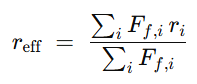


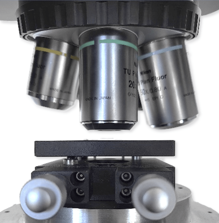
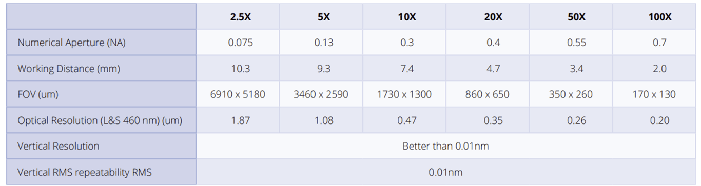
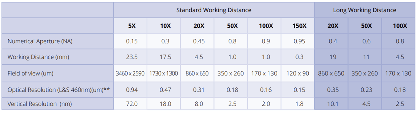
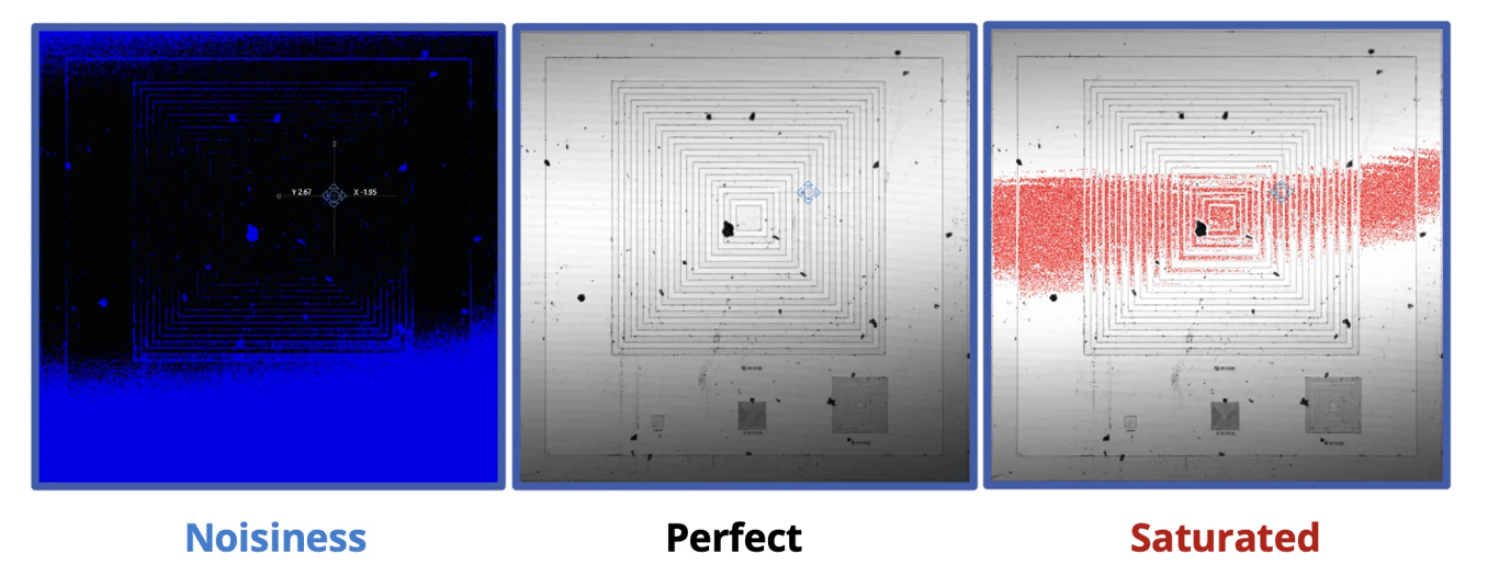

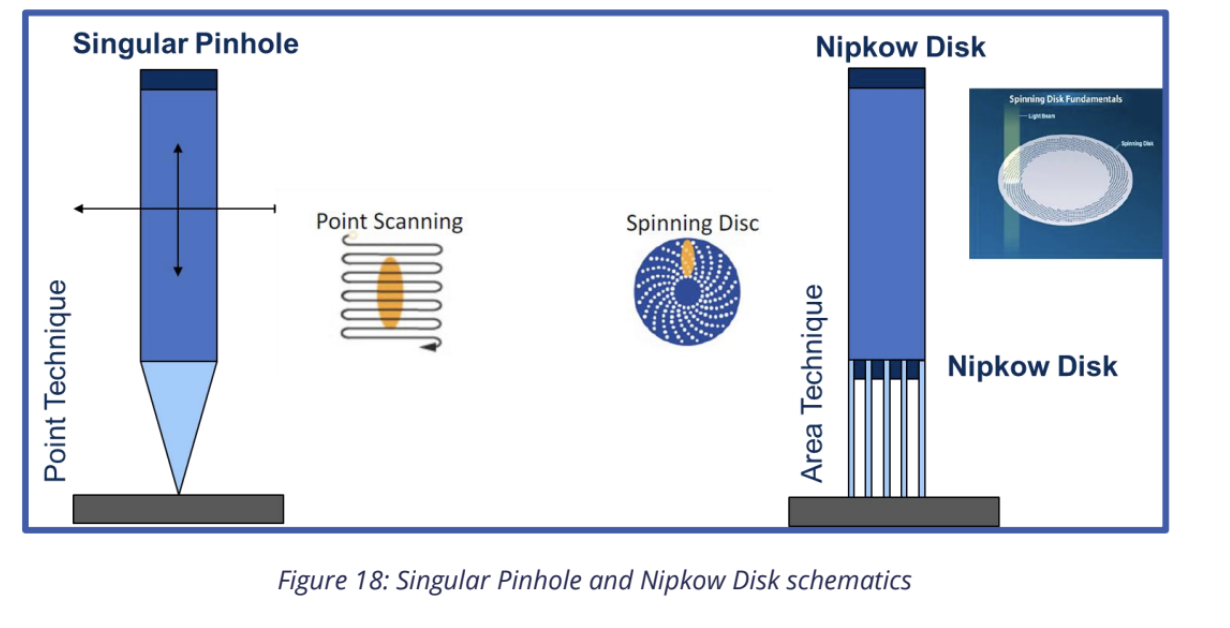


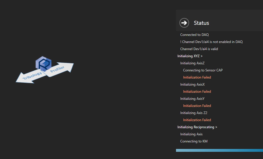

 Made with Bullet