If there the drive is not currently in place ,follow theses step below.
Otherwise please continue to the next step.
As shown above, the drive is installed on the stage.
Direct Rotary Drive Installation Step
Additional animation instructions
Route the drive cable through the X Y stage.
Position and insert the motor drive through the stage.
Orient the drive so the green sensor port faces the right side.
Secure the drive with 7 x SHCS 8-32 X .625" long screws (310-280-05 / BM310280-09)
Confirm that the alignment pin is seated correctly.
Connect the 2 cables on the slot on the right, behind the frame (the Motor Power Chord and the Encoder Chord).
⚠️
Always power off the instrument before connecting cables or installing any load cell or accessory.
If Integrated module
In certain configurations—particularly when there are requirements for speed and/or torque—a module with an integrated motor has been recommended.
The difference, therefore, is that to change modules (from reciprocating to rotary, for example), it is necessary to uninstall the module with it motor from the stage.
Open the upper back door of the MFT-5000.
Insert the motor drive on the stage.
Secure it with 6 x 8-32 x .375” BM310280-05 9/64
Connect the 2 cables on the slot behind the right frame.
Skip the next step.
Rotary
Install the Rotary Drive
Align the rotary drive with the mounting holes.
⚠️
Ensure that the black connector underneath the module is facing left so it properly aligns and connects with the green connector on the base.
Secure using 6 x 8-32 screws (Part No. BM310280-5) with 9/64" Allen key.
Rotary Options
Remove the Rotary Table
Using a 9/64" Allen key, remove the existing sample holder disk to prepare for the chamber installation.
Remove the thread adapter and pin from the rotary table disk.
The pin is a 0.094” x 0.375” dowel pin, part number BM280103-04. The thread adapter is part number BM430001.
Mount the Lower Extension
Align the lower extension with its mounting position.
Secure it using three 8-32 screws (BM310280-4) and a 9/64" Allen key.
Re-Mount the Rotary Table
Insert a long ¼-20 bolt in the center of the rotary table to help lower and position the table into the chamber.
Place the rotary table inside the chamber.
Once seated, remove the temporary screw and re-screw the three rotary table screws with the 9/64" Allen key.
Mount the Sample Disk
Place the sample disk on the holder.
Fasten with one 4-40 screw using a 5/32" Allen key.
Linear
Drive -
Linear Reciprocating Drive Installation
Position the reciprocating drive on the base.
⚠️
Ensure that the black connector below the module is properly aligned and connects with the green connector on the base.
Use two 8-32 screws (BM310280-12) to secure the reciprocating drive.
Technical Linear Drive Specification
Adjustable Stroke length: 0.1-30 mm
Frequency: 0.1-80 Hz ( 80 Hz @ 1 mm, 60 Hz @ 2 mm, 20 Hz @ 25 mm).
⚠️
The maximum allowable frequency is determined by the current stroke length. The respective limits must not be exceeded.
Some reciprocating drives are not fully covered by this specification, e.g., SPN04316 – up to 15 Hz. Please refer to your packaging list if unsure or unaware of this information, or contact Rtec Support for assistance.
(Option) LVDT Linear Encoder Range: 25.4 mm (+/- 12.7 mm); Resolution: 1 um
ℹ️
When using the reciprocating system in combination with the LVDT, the stroke length limitation becomes 25.4 mm. The stroke length cannot be measured beyond this value.
Fast reciprocating drive - Adjustable Stroke length: 0.1-30 mm; Frequency:0.1-80 Hz ( 80Hz @ 1mm, 60hz @ 2mm,40 Hz @ 13 mm ,20 Hz @ 25mm ,10Hz+ @ 30mm, ) With LVDT Linear Encoder Range: 25.4 mm (+/- 12.7 mm); Resolution: 1 um
Adjusting the Stroke Length
⚠️
Please remember that the maximum frequency varies according to the stroke length. ( 80 Hz @ 1 mm, 60 Hz @ 2 mm, 20 Hz @ 25 mm).
When using the reciprocating system in combination with the LVDT, the stroke length limitation becomes 25.4 mm. The stroke length cannot be accurately measured or guaranteed beyond this value.
On the MFT Software , disable the drive by clicking on the ON button.
ℹ️
Click on “ON” to switch off the motion. The module must be “OFF”. The drive must be disabled in order to freely move the reciprocating and get access to the adjustment screws.
Drive disabled, turn the central shaft until the stroke adjusting assembly appears through the front opening of the module.
Animation example
Using a 5/64” Allen wrench, loosen the brake screws on both sides
Animation example
Insert a 9/64” Allen wrench into the center adjustment screw to adjust the stroke length.
ℹ️
Turn clockwise (right) to decrease stroke length. Turn counterclockwise (left) to increase stroke length.
Measure the amplitude with the LVDT if available in your configuration, a ruler or a dial gauge while the drive motion is on.
ℹ️
Manual measurements of the reciprocating amplitude may differ slightly from the drive motion amplitude. For accurate stroke length, measure with a dial gauge while the drive is running, or use the LVDT sensor if available.
After adjusting, re-tighten the brakes with the 5/64” Allen wrench.
Connecting the LVDT {{if lvdt,reci,srv}}
ℹ️
This feature is optional and included only in systems purchased with the LVDT attachment for displacement measurement (SPN04325)
Connect the LVDT cable to the port located at the back of the drive.
Attach the Universal Sample Holder
Place the universal sample holder on top of the reciprocating drive
Tighten the captive screws using a 7/64" Allen key.
Insert the sample
Position the sample into the universal holder.
ℹ️
Max sample width: 1.61” (4.089cm).
Other than the width, the rectangular sample has no specific size requirements.
(Optional) You can also loosen the two nuts first to fit the sample size before.
Secure the sample in place using an 8/32" Allen key
Linear Options
Install the Chamber Stands
Position the two support stands, one at the front and one at the rear of the drive.
Secure each stand using one 10-32 screw (BM310320-12).
Tighten with a 5/32" Allen key.
Update the configuration - List
Located in:
Type:
Options to select:
Sensors
Fz
Your Sensor Range
Sensors
Fx
Your Sensor Range
Sensors
Fx
Any Sensor Range - Not used for COF calculations.
Sensors
TS
Your Sensor Range
Sensors
CAP
Your Sensor Range
Sensors
AE
Your Sensor Range
Sensors
LVDT-Position
Your Sensor Range
Sensors
LVDT-Stroke
Your Sensor Range
Sensors
ECR
Your Sensor Range
Sensors
HiperECR
Your Sensor Range
Sensors
HiperV
Your Sensor Range
Sensors
HiperI
Your Sensor Range
Sensors
Analog Input 1
Your Sensor Range
Sensors
Analog Input 2
Your Sensor Range
Sensors
6D
Your Sensor Range
XYZ
XYZ
XYZ: XYZ Stage
Z: Only Z Stage
Lower Drive
AutoDrive
Select for current Drive generations
Lower Drive
Rotary
Select for previous Drive generations
Lower Drive
Reciprocating
Select for previous Drive generations
Lower Drive
BlockOnRing
Select for previous Drive generations
Lower Drive
4Ball
Select for previous Drive generations
Lower Drive
Indenter
Select for Indenter Head
Lower Drive
VoiceCoil
Select for VoiceCoil
Lower Drive
TapTorque
Select for TapTorque Module
Lower Drive
Scratch
Select for TapTorque Table Module
Lower Drive
TwinRoller
Select for TwinRoller Module
Temperature Control
RTC
Rotary-75C:
Use for 0-75°C
Rotary-180C:
Use for 75-180°C
Rotary-500C:
Use for 180-500°C
Rotary-1000C:
Use for 500-1000°C
Rotary-1200C:
Use for 1000-1200°C
Reciprocating-75C:
Use for 0-75°C
Reciprocating-180C:
Use for 75-180°C
Reciprocating-500C:
Use for 180-500°C
Reciprocating-1000C:
Use for 500-1000°C
Reciprocating-1200C:
Use for 1000-1200°C
BOR-75C:
Use for 0-75°C
BOR-180C:
Use for 75-180°C
BOR-500C:
Use for 180-500°C
MTM-180C:
Use for 75-180°C
4Ball-180C:
Use for 0-180°C
Stage-250C:
Use for 0-250°C
VoiceCoil-60C:
Use for 0-60°C
VoiceCoil-75C:
Use for 60-75°C
VoiceCoil-180C:
Use for 75-180°C
Temperature Control
Chiller-Julabo
-40°C
Temperature Control
Chiller-ThermoFisher
-40°C to +150°C
Coefficient Of Friction
COF
COF
COF-Tz
COF-TS
COF-Piezo
COF-Piezo-RMS
Vacuum
Vacuum
Vacuum
Humidity
Humidity
Humidity
Electrochemical Measurement Systems
Keithley
Keithley 2450
Keithley 2750
Electrochemical Measurement Systems
Admiral
Admiral
Electrochemical Measurement Systems
Versastat
Versastat
Electrochemical Measurement Systems
Modulab
Modulab
Electrochemical Measurement Systems
GwInstek
GwInstek
Analog Ouput
Analog Ouput
Analog Ouput
Add Steps - List
Add a Keithley Measurement
In the same Standard step, click on E-TEST.
Click on Idle.
Select 4-Wire Measurement.
Add a Voltage Control on the Potentiostat
In the same Standard step, click on E-TEST.
Click on Idle.
Select Voltage Control.
Enter the desired voltage applied during the step.
Add a Rotary Radius [rota]
My tester doesn't have XY motorization
Manually adjust the Upper holder Y Radius and ignore this step
To adjust the y radius you need to manually turn the knob to the desired radius.
The center of the Y radius setup being the 25mm mark, you can adjust the radius to +-25mm.
Click the drop-down menu and select Reposition.
Click ADD a new step.
Click ADD a new item.
Click 3 times on Z.Velocity to get the dropdown menu
Click on Y.Position.
Press ENTER.
Enter the radius desired in Value. ex: 5 mm
For more information
⚠️
Most Rtec-Instruments load cells are designed to measure friction along the X-axis (Fx).
Because of this, it’s important to always set Y to a nominal value and X = 0. This ensures that all friction forces appear only along the X-axis, where the sensor can detect them.
If you adjust the radius along X, the friction force will shift to the Y direction (Fy). In that case, the load cell will not be able to measure it correctly, and it could even cause damage to the sensor.
Add a Standard Step [!scr,ind]
For more information
Principle of the STANDARD Step:
A standard step can combine multiple axis and module activations, such as applying a force (Z stage), enabling motion (Drive function), and heating the sample (Temperature function for chambers).
During this combinated step, the force is first applied and stabilized. Then, if a heating chamber is used, the defined temperature is reached. Finally, the drive type of motion drive is activated and the duration starts.(unless the engage parameters are modified).
Standard Individual step modification window
Part 1: Duration
Duration window
Duration of the step
In this window you can control the duration of the step.
The highlighted button allows the user to automatically calculate the duration of the step if the parameters selected offers to do so with a defined duration of a single repetition and certain number of repetitions (Slide for example)
By default, the logging and time duration start after the force is reached. (see Waiting for force/temperature to settle further)
Part 2: Reset
Reset window
In this window you can reset the value of Fx at the beginning of the step. If it is unchecked, the Fx value will not be subjected to any reset.
This option is necessary to be pressed only when there is an offset of the Fx value at the beginning of the test (1D+1D arm), it will create issues in most cases when using a 2D Load Cell.
Part 3: Data Logging
Data logging window
Checking “Log during this step” will record the test data during the step. If it remains unchecked, no data will be logged for this step.
In case the user wants to divide the data logging into smaller periods, he can modify the values of “Log Period” and “Log Interval”.
Log period (seconds): The duration of the log period.
Log Interval (seconds): The duration of the interval between 2 log periods.
Part 4: Force
Force window
Force options:
Constant: The step is run at a constant value of force. For example: 10N.
Linear: The step is run in linearly increasing or decreasing force for the entire step duration. For example: 5N to 20N. So, the slope's steepness will depend on the duration of the time period.
Undefined: No force control and regulation. Z drive shall remain at the same position throughout the step, this is the equivalent of the Idle state. Use this options if you only use the drive or the temperature during this step for example.
⚠️
The Z-Axis will reach out for a contact when applying a constant force of 0 N as opposed to the undefined option.
Each force are defined for each step, this aspect must be taken in consideration, meaning that the same force must be defined each step to keep applying the desired force throughout the run-test.
Tracking : Adjusting the reaction time
Tracking options:
Low: Reduces the Fz reaction time and adjustment intensity. Only to be used if the standard option is adjusting too strongly to a slow Fz evolution (Tests with fast and high Z displacement).
Standard: To be used in most cases.
High: Increases the Fz reaction time and adjustment intensity. Only to be used if the standard option is adjusting too slowly to a rapid Fz evolution (Tests with fast and high Z displacement).
We highly recommend to use the Standard tracking. However, if the tracking of the force is not satisfactory, you can try other possibilities or contact Rtec customer service if you cannot obtain a satisfactory tracking of the force
Click the drop-down menu and select Standard.
Click ADD a new step.
Define the duration of the step in the DURATION Section.
Define a constant or linear force within the range of the sensors and suspension.
Press ENTER.
⚠️
Remember to define values below the limits of your load cell and suspension.
(Refer to the load cell manual, suspension section for help)
Activate the X Axis [stat,scr]
Standard (tribology / scratch) measurements can be performed by using the X-stage. This does not include an automated pre- and post-scanning features or defining touch force or approach speed. When clicking on “standard”, you can create a recipe. This type of measurement can be selected when using the “universal ball/pin holder” instead of a standard Rockwell-C indenter.
[scr]
In the same Step, click on X AXIS.
Click on Idle to unroll the list.
Select Slide.
Insert the Distance (Displacement amplitude). Ex: 5 mm
Insert the Velocity, press Enter. Ex: 10 mm/s
Leave Acceleration defaut value.
Default Motorized Table specifications (subject to customization):
Default MFT-2000 Motorized Table specifications:
X Max travel: 150 mm / Up to 50 mm/s
Y Max travel: 200 mm / Up to 50 mm/s
Default MFT-5000 Motorized Table specifications:
X Max travel: 130 mm / 0.001-6 mm/s
Y Max travel: 270 mm / 0.001-50 mm/s
Default SMT-5000 Motorized Table specifications:
X Max travel: 150 mm / 0.001-50 mm/s
Y Max travel: 150 mm / 0.001-50 mm/s
For more information
X axis motion
In this parameter, the user can command an action of the X axis for the step.
Idle: X axis does not move the during the step.
Cycle: Triangular motion along the X axis for the entered distance and number of cycles.
Distance: Amplitude of the X-axis displacement.
Velocity (rpm): Final velocity of displacement after the acceleration phase.
Acceleration (s): Acceleration phase duration.
ℹ️
The previous position of the X table is used as the origin. The distance setting will thus be the distance from the previous X position.
For example, if the X position is 0 and the Amplitude is set to -2mm, the axis will create a triangular movement between X=[0;-2mm]
Slide: Moves the X axis for the entered distance relative to the previous position (positive and negative as shown on the X, Y platform).
Activate the Drive [!scr]
For more information
Drive motion
The action type might change based on the drive selected.
Idle: If this action is selected, the drive doesn’t move during this step.
Cycle:Oscillates the drive in counter and clockwise directions.
Revolution: Number of revolutions before it changes direction.
ℹ️
If the number of revolutions entered is below 1, the rotary drive will realize a reciprocating-like rotary movement.
Velocity (rpm): Final velocity of displacement after the acceleration phase.
Acceleration (s): Acceleration phase duration.
Slide: Moves the drive for a fixed number of revolutions.
Revolution: Number of revolutions to be realized.
Velocity (rpm/Hz): Final velocity of displacement after the acceleration phase.
Acceleration (s): Acceleration phase duration.
Continuous: Moves the drive at constant velocity in counter or clockwise direction.
Direction: CW for clockwise, CCW for counterclockwise direction.
Velocity (rpm/Hz): Final velocity of displacement after the acceleration phase.
Acceleration (s): Acceleration phase duration.
Move to Angle: Moves the drive to a nominal angle of the shaft
In the same Standard Step, click on DRIVE.
Click on Idle to unroll the list.
Select Continous.
Insert the Velocity. Ex: 500 Rpm or 10hz
Insert Acceleration and Deceleration time (or leave default). Ex: 5s
Activate the Temperature Chamber [heat,cool]
In the same Standard step, click on TEMPERATURE.
Click on Idle
Select Lower Chamber.
Enter the C° temperature to reach for.
Press ENTER.
This temperature will be reach at the start of the step.
Click NEXT to go to the next Window.
When Only Idle appear → The Temperature module is not properly selected → see Update the Components.
ℹ️
Idle: No temperature chamber action is done during the step.
Upper Heater: Sets the desired temperature of the upper heater (if available)
Lower Chamber: Sets the desired temperature of the lower chamber (if available)
Lower &Upper: Sets the temperature of the upper and lower chambers (if available)
Stop: Remove a previous defined temperature setpoint during the test.
Enter the 4Ball Effective Radius {{if upper-rotary,4ball}}
In the same Standard step, click on the free area next to Effective Radius(mm).
Enter 4.49.
Help
Enter the Effective Radius [bor,urota,4ball]
The value inserted in this animation is an example.
In the same Standard step, click on the free area next to Effective Radius(mm).
Enter 34.93 for the default ring.(Refer to the Help section for other samples).
{{if bor}}
Enter 4.49 (mm). {{if 4ball}}
Help
BOR Effective Radius Calculations
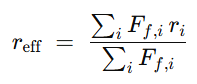
For Block On Ring test, the Friction Coefficient (COF-Torque) is calculated using the effective radius entered in the “Radius” field of the previous window.
The effective radius of the block on ring depends on the amount of contact areas where the friction occurs:
Ring test: Only one single contact point at the radius of the ring.
“Radius” = Radius of the ring (mm).
Bearing test: Two contact points: One between the balls and the inner ring and a second one between the balls and the outer ring.
“Radius” = Effective radius of the 2 contact areas (mm).
The effective radius can be estimated as follows:
Ff,i being the friction force at a specific contact radius.
{{if bor}}
{{if 4ball}}
4Ball Effective Radius Calculations
Four 12.7mm (0.5”) balls are used in the 4Ball test. The following calculation explains why an effective radius of 4.49 needs to be selected in the software for this specific test method:
The radius selected will be defined for the whole recipe and registered in the sample information section.
Add a Scratch Step
Click the drop-down menu and select Scratch.
Click ADD on the bottom left.
Click On 0.1 and enter the scratch starting force.
Click on 10 and enter the scratch ending force.
Click on the circle next to Load Rate to automatically calculate it.
Enter the Scratch Velocity.
Enter the Scratch Distance.
Help
Recommendations:
Starting Force = 0.1N
Velocity = 30 mm/min
Distance = 5 mm/min
Load Rate < 100 N/min
For more information
Scratch step
Scratch step window
Part 1: Scratch parameters
Mode
You can choose between different scratch techniques:
Scratch Only: After finding the contact point, realizes a single scratch during which it records the selected parameters.
This type of scratch test is mostly used for scratch tests with a profilometer. The profilometer is the most efficient at analyzing a final scratched surface.
Pre-Scan/Post-Scan: Realizes a pre-scan at very low force along the scratch length to analyze the original surface. After this pre-scan, it realizes the scratch. Finally, following the scratch it realizes a post-scan at very low force along the scratch length to analyze the final scratched surface.
This type of scratch test with a pre and post scan is mostly used for scratch tests without a profilometer to analyze the final scratched surface.
It is recommended to obtain the true scratch depth (not affected by any tilt or curvature on the sample surface) and to measure the residual scratch depth. Residual scratch depth is the profile of the scratch which remains after the scratch is completed. Due to self-healing and viscoelastic properties, the residual scratch profile may differ from the depth during the scratch.
Force (N)
There are different possibilities of force applications:
Constant: Applies a constant force throughout the displacement.
It is recommended for mar resistance testing (at low force)
Linear: Applies a linear force starting from the force entered in the left to the force entered in the right. (It only works for positive linear force application?)
For coating adhesion measurements it is suggested to use linear increasing loading.
Calculate
In this part, you need to enter 2 parameters to determine the velocity, distance and load rate of your scratch test.
It is possible to modify 2 of the 3 parameters as they are interdependent. By clicking on the circle at the left side of the parameter, it will lock its value and automatically calculate it based on the 2 other parameters.
We recommend to use a load rate below 150N/min. Using a load rate higher than this value will reduce the quality of the Fz tracking.
Part 2: Scratch scan parameters
Scratch scan parameters schematics
You can arrange the 2 parameters of the pre and post-scans:
Back Scan (mm): The length of the scan on the opposite direction of the scratch (the dotted line before the scratch solid line).
Scan Force (N): The force applied to analyze the surface during the pre and post scan.
We recommend to use a Back Scan distance of 0,2mm and a scan force of 0,1N. It is recommended to keep the scan-force limited. Setting the scan force too low may result in false contact detection during the indenter approach phase.
Part 3: Scratch sample approach
The Touch Force can be modified here. It corresponds to the force the tip is applying when finding the surface.
We recommend to use 0,1N. A too low touch force may result in a false contact detection during the indenter-sample approach phase. Thus, if the load cell does not reach the sample when starting a scratch test, it is highly likely that you need to increase the value of the touch force.
More settings
You have the possibility to adapt settings to modify the scratch test settings to your specific application. To do so, please refer to part 6.4.
Add an Indentation Step
Add a Traction Step
Add a Stribeck Step
Introduce the components - List
Modules with Rotation
Rotary, Block On Ring, Upper Rotary (4Ball, TapTorque)
Sampling rate (Hz) = max. Rpm/2 Averaging = 5.
Ex: 1 Khz for a drive velocity of 2000RPM
Modules with Reciprocating motion
X, Y Stage Reciprocating, Linear Reciprocating and VoiceCoil
for ASTM G99 standard: select appropriate samples according to.
Home the system and place the upper sample above the lower sample.
Create a new recipe, then follow the desired recipe steps below.
Simple rotary test
In the new recipe, Add the first Reposition Step
Sensor.Reset Fz: 1
Sensor.Reset Fx: 1
Y.Position: Your test radius value
X.Position: 0
⚠️
X axis Position must be at 0 for rotary tests
Most Rtec-Instruments load cells are designed to measure friction along the X-axis (Fx).
Because of this, it’s important to always set Y to a nominal value and X = 0. This ensures that all friction forces appear only along the X-axis, where the sensor can detect them.
If you adjust the radius along X, the friction force will shift to the Y direction (Fy). In that case, the load cell will not be able to measure it correctly, and it could even cause damage to the sensor.
Disengage Z: ✅
(Optional) rename it : Reset Sensor & Position
Add a Standard Rotary Step along with the followings drive motion.
Add a Standard Rotary Step
Duration: Your value
Force: Your value
Logging: ✅
Activate one of the following drive motion.
Continuous Rotary
Drive: Continuous
Parameters to be determined.
Reciprocating-like Rotary
Drive: Cycle
Revolutions: 0 to 1
Other parameters to be determined.
Spiral Rotary
Drive: Continuous
Parameters to be determined.
Y Axis: Slide
Distance: Smaller than the sample radius and larger than track diameter (to avoid passing twice on the same area)
(Optional) Add an Imaging Step.
Add a Loop/Delay Step from the Reposition Step 1.
Go to Data Logging
Sampling rate (Hz): max. RPM/2
Averaging: 5
Record: Fz & Fz, COF, Rotary Angle/Velocity Y position
Brake Pad : Rotary decelerating test
Reset Sensor & Position
Add a Reposition step
Sensor.Reset Fz: 1
Sensor.Reset Fx: 1
Y.Position: Your value
X.Position: 0
Disengage Z: ✅
Apply Desired Force
Add a Standard Step
Duration: 5 seconds
Force:Desired braking force.
Logging: No
Lift Up
Add a Reposition Step
Z.Velocity: 4mm/s
Z.Offset: 5mm
Disengage Z: ❌
Increase if the upper holder still touches the sample after this step.
Set Initial Velocity
Add a Custom Step
Using a custom step instead of a standard step is necessary to avoid that the motor stops during the following reposition step.
Continuous
Velocity: To be determined Initial breaking velocity.
Touch Down
Add a Reposition Step
Z.Velocity: 4mm/s
Z.Offset: -5mm (Or the Value entered previously)
Disengage Z: ❌
Breaking Duration
Add a Standard Step
Duration: Your Braking duration
Force: Your Braking force
Drive: Continuous
Velocity: Final Braking Velocity
Deceleration: Deceleration time between Initial speed (in Custom step) and final speed (in this standard step).
Optional: Temperature Verification
Add a Standard Step
Duration: 2 hours
Force: Undefined
Go to Recipe Parameters → Advanced
Abort_STEP
Temperature.IRT
<
Your temperature threshold to resume testing
Add a Loop/Delay Step from Step 1 with Disengage Z.
If you are simply interested in controlling the rotary decelerating time, you can use the same recipe and remove steps 3 and 5.
Go to Data Logging
Parameters
Sampling rate (Hz): max. RPM/2
Averaging: 5
Record:
Fz & Fx (or Tz)
COF
Rotary Angle/Velocity
Y position
Rtec Instruments ASTM G99 Test Protocol
⚠️
This procedure is based on the ASTM G99 Standard Test Method for Wear Testing with a Pin-on-Disk Apparatus. The full standard is available from ASTM International (www.astm.org). This document is not a substitute for the official ASTM G99 standard.
Summary of Standard
This test method covers a laboratory procedure for determining the wear of materials during sliding using a pin-on-disk apparatus. Materials are tested in pairs under nominally non-abrasive conditions. For the pin-on-disk wear test, two specimens are required. One, a pin or ball that is positioned perpendicular to the other, usually a flat circular disk. The tester causes stationary pin/ball to press against the rotating disk at a known force and speed. During the test COF, friction, wear etc. parameters are measured and reported.
Pin On Disk Setup
This standard is applicable to metallic samples, non metallic, polymers, ceramics, composite materials etc.
Procedure
Check the hardware installation
After having followed the basic step-by-step software:
The upper load cell and lower rotary modules are properly installed following their respective steps.
The additional thermocouple must be connected in place at a location close to the wearing contact as indicated in ASTM G99. It is recommended to attach it to close to the ball as it is stationary during the test.
The software configuration have been followed, therefore, the temperature component is selected.
Right Click on the .rx file attached above, click on Save Link As and save the file to any location on the PC.
Start MFT, click on “Expert Mode” and press Add the recipe
Select saving directory and select the recipe downloaded.
Adjust the recipe parameters
Only Modify explicitely stated steps
Sensors Reset & Sample Positioning
Modify Reposition Step
Y.Position: Enter Test radius. G99 Guide: 16mm (32mm diameter)
Initial Force Application
Modify Standard Step
Force: Enter Test Force G99 Guide: 10N
ASTM G99 Test
Modify Standard Step
Duration: change to 100hrs
Force: Enter Test Force (Same as Step 2) G99 Guide: 10N
Drive: Continuous Linear Velocity (or Constant Linear Velocity when no XY table)
Linear Velocity (mm/s): Enter desired linear velocity
G99 Guide: 100 mm/s (0.1m/s)
Direction: To be determined
Modify the limit condition
Go to Recipe Parameters → Advanced
Click on Step 3
Click on the limit condition on the right
Change the limit value to the amount of revolutions you desire
G99 Guide: 10000 revs (1000m at 0.1m/s)
Go to Sample Info.
Parameters
Upper & Lower Sample information
Material Type
Form
Processing Treatments
Surface Finish
Specimen preparation procedures
Environment information
Temperature
Relative Humidity
Interfacial Media
Go to Data Logging
Logging Parameters
Sampling rate (Hz): Modify to max RPM/2
Data Collected:
Keep following items, add or remove if necessary:
Fz, Fx, COF, Y Position, Radius value , Rotary Position
,Accumulated Revolutions ,Rotary Linear Velocity (Sliding speed between surfaces), Temp-2
Temperature of one specimen close to the contact (using additional thermocouple)
Run the Recipe
Home the system and start the test in the Run tab.
After test completion, clean both upper and lower samples to remove any debris.
Measure the wear volume on the sample and pin.
Please refer to the Performing an Image Acquisition step for more
Rtec-Instruments Lambda Imaging Head provides accurate data for full wear analysis (stitching) or cross section wear area (single image).
Calculate Measurement uncertainty and perform other analysis by following ASTM G99 documentation.
Rtec Instruments Data Results
Universal ball Holder
440-C Stainless Steel Ball, Dia. 9mm
Stainless Steel Disk (2 inch)
Comparative test at 3 separate laboratories on G99 procedure.
Reciprocating test
Clean and Mount upper and lower samples.
Home the system and place the upper sample above the lower sample.
Physically adjust the stroke.
Create a new recipe
Reciprocating module test
Add a Reposition step:
Sensor.Reset Fz: 1
Sensor.Reset Fx: 1
Disengage Z: ✅
Add a Standard step:
Duration: To be determined
Force: To be determined
Drive: Continuous
Parameters to be determined.
Logging: ✅
Optional with Imaging Head:
Add a Reposition step: Shaft goes to a specific angle, image always at the same part of the sample.
Move.Angle: 0
Add an Inline imaging step:
Inline Calibration to be performed
Image parameters to be selected (Top / Bottom / Objective used…)
Image type and parameters to be selected
Add a Reposition Step
Y.Offset: 3mm Moves the sample outside the existing track.
⚠️
When performing an Offset, make sure that it will not reach out of the sample during the whole recipe loops.
Add a Loop/Delay:
From: Reposition step
For: To be determined Number of iterations (including first one)
In Data Logging:
Sampling rate (Hz): max. Freq (Hz)*30
Averaging: 2
Record:
Fz & Fz
COF
Rotary Angle/Velocity
Y position
X-axis Reciprocating test
Add a Reposition step:
Sensor.Reset Fz: 1
Sensor.Reset Fx: 1
Disengage Z: ✅
Add a Standard step:
Duration: To be determined
Force: To be determined
Drive: X axis
⚠️
Only X-axis tests can be performed on most load cells.
Most Rtec-Instruments load cells are designed to measure friction along the X-axis (Fx).
Because of this, it’s important to always realize a X-axis reciprocating motion. This ensures that all friction forces appear only along the X-axis, where the sensor can detect them.
If you active the Y motion, the friction force will shift to the Y direction (Fy). In that case, the load cell will not be able to measure it correctly, and it could even cause damage to the sensor.
Parameters to be determined.
Logging: ✅
Optional with Imaging Head:
Add a Reposition step: Shaft goes to a specific angle, image always at the same part of the sample.
Move.Angle: 0
Add an Inline imaging step:
Inline Calibration to be performed
Image parameters to be selected (Top / Bottom / Objective used…)
Image type and parameters to be selected
Add a Reposition Step
Y.Offset: 3mm Moves the sample outside the existing track.
⚠️
When performing an Offset, make sure that it will not reach out of the sample during the whole recipe loops.
Add a Loop/Delay:
From: Reposition step
For: To be determined Number of iterations (including first one)
In Data Logging:
Sampling rate (Hz): max. Freq (Hz)*30
Averaging: 2
Record:
Fz & Fz
COF
Rotary Angle/Velocity
Y position
Rtec Instruments ASTM G133 Test Protocole
Not available - recipe created
Block On Ring test
Clean and Mount upper and lower samples.
Home the system and place the upper sample above the lower sample.
Create a new recipe, then follow the desired recipe steps below.
Simple Block On Ring test
In the new recipe, Add the first Reposition Step
Sensor.Reset Fz: 1
Sensor.Reset Fx: 1
Disengage Z: ✅
(Optional) rename it : Reset Sensor & Position
Add a Standard Step along with the followings drive motion.
Add a Standard Step
Duration: Your value
Force: Your value
Logging: ✅
Activate one of the following drive motion.
Back and Forth Block On Ring
Drive: Cycle
Revolutions: 0 to 1
Other parameters to be determined.
Continuous Block On Ring
Drive: Continuous
Parameters to be determined.
(Optional) Add an Imaging Step.
Add a Loop/Delay Step from the Reposition Step 2.
Go to Data Logging
Sampling rate (Hz): max. RPM/2
Averaging: 5
Record: Fz & Fz, COF, BOR Angle/Velocity
Rtec Instruments ASTM G77 Test Protocol
Not available - recipe created
Rtec Instruments ASTM G137 Test Protocol
Not available
Rtec Instruments ASTM G176 Test Protocol
Not available - recipe created
Rtec Instruments ISO 7148 Test Protocol
Not available
TriboCorrosion Test
Tribocorrosion evaluates how mechanical wear and electrochemical corrosion interact when a material is exposed to both sliding contact and a corrosive medium.
It simulates real service conditions to assess film stability, material loss, and wear–corrosion synergy.
Test Types:
Standard Tribocorrosion Test (OCP): No applied potential — measures natural potential (E(t)) to study film breakdown and repassivation.
Anodic Tribocorrosion Test: Constant applied potential — monitors current (I(t)) to assess wear–corrosion under controlled anodic protection conditions.
Standard Tribocorrosion Test
OCP test
This recipe evaluates natural corrosion and film repassivation behavior under sliding.
Polish a new sample, clean sequentially with acetone, isopropanol, and deionized water, dry with compressed air, then mount it in the tribo-corrosion cell and fill with fresh electrolyte.
Create a new recipe.
Add a Standard step (OCP Stabilization)
Duration: 15-30 mins (or until potential drift < 1–2 mV/min)
Force: Undefined
Drive: None
E-Test: None
Logging: Yes
Add a Standard step (Drive ON)
Duration: To be determined
Force: To be determined
Drive: Reciprocating Parameters to be determined
E-Test: None
Logging: Yes
Add a Standard step (Drive OFF)
Duration: To be determined
Force: Undefined
Drive: None
E-Test: None
Logging: Yes
Add a loop
From:Drive ON Step
For: To be determined
Logging: No
In Data Logging
Sampling rate (Hz): max. Freq (Hz)*30
Averaging: 2.
Record: “weVoltage”, “Current” and other tribological parameters.
Open Rtec Insight and compare the weVoltage [E(t)] between the sliding and idle steps to determine:
Potential Drop between no contact and sliding.
Recovery kinetics of repassivation. (see Help)
Retrieve OCP value for recipe 2.
Take a profilometer image of the wear mark to determine T:
T = Total material volume lost under mechanical and corrosion influence
Help
Determine Steps duration:
Focus on kinetics (how quickly the surface film breaks down and repassivates):
Drive ON: 60–120 s
Drive OFF: 180–300 s.
Focus on steady wear (long-term equilibrium behavior under sustained mechanical action):
Drive ON: 180–300 s
Drive OFF: 90–120 s.
Determine Reciprocating Parameters:
Define the reciprocating motion parameters (stroke length, frequency) that provide consistent mechanical contact and realistic wear conditions for your specific tribo-corrosion testing.
Parameter
Symbol
Typical Range
Stroke length
L
1–5 mm
Frequency
f
0.5–5 Hz
Normal load
Fₙ
Material-dependent
Repassivation kinetics (τ) — how to compute:
Extract the repassivation time constant τ by fitting the weVoltage curve using:
E(t)=E∞−(E∞−Emin)∗exp(−t/τ)
E(t): Potential at time t after sliding stops. Emin: The lowest potential right when sliding stops (most active state).
E∞: The final potential after full recovery (steady passive state).
t: Time after sliding stops.
τ: Time constant (s); after t=τ, recovery ≈63% complete
Cathodic Protection test
This recipe evaluates mechanical wear under suppressed corrosion to isolate W0.
Reuse the same sample on a new wear track (positioning the upper holder in a new location), clean it sequentially with acetone, isopropanol, and deionized water, dry with compressed air, then mount it in the tribo-corrosion cell and fill with fresh electrolyte.
Create a new recipe.
Add a Standard step (OCP Stabilization)
Duration: 15-30 mins (or until drift < 1–2 mV/min)
Force: Undefined
Drive: None
E-Test: None
Logging: Yes
Add a Standard step (Conditioning)
Duration: 10-15 mins
Force: Undefined
Drive: None
E-Test: OCP - 350mV OCP Value from Recipe 1
Logging: Yes
Add a Standard step (Drive ON)
Duration:Same as Drive ON in OCP test.
Force:Same as Drive ON in OCP test.
Drive: Reciprocating Same parameters as Drive ON in OCP test.
E-Test: OCP - 350mV OCP Value from Recipe 1
Logging: Yes
Add a Standard step (Drive OFF)
Duration:Same as Drive OFF in OCP test.
Force: Undefined
Drive: None
E-Test: OCP - 350mV OCP Value from Recipe 1
Logging: Yes
Add a loop
From:Drive ON Step
For:Same as OCP test
Logging: No
In Data Logging
Sampling rate (Hz): max. Freq (Hz)*30
Averaging: 2.
Record: “weVoltage”, “Current” and other tribological parameters.
Open Rtec Insight and compare the weVoltage [E(t)] between the sliding and idle steps to determine:
Stability of cathodic protection during sliding (verify current remains constant and small).
Absence of hydrogen evolution: confirm no large current spikes or oscillations.
If current fluctuates strongly or hydrogen bubbles appear, reduce the applied cathodic offset (use OCP − 300 mV or OCP − 250 mV).
Take a profilometer image of the wear mark to determine W0. W0: Total material volume lost without corrosion influence.
Tafel Plot
Open “Squidstat User Interface.exe”.
If prompted to update firmware → click “Postpone”
⚠️
Do not update Admiral Firmware if asked to. MFT software communication would be permanently lost by doing so.
Click on Linear Sweep Voltammetry
Change the Parameters to:
Select the Admiral Potentiostat.
Run the test
Plot:
log(I)=f(E)
Obtain E_corr and I_corr
Determine C0 by using the following formula:
C0=(Icorr∗t∗M)/(n∗F∗ρ)
Where:
t: Time of exposure (s): Total sliding duration (Drive ON periods) for the tribo-corrosion (Recipe 1 & 2) tests.
n: Valence number: Number of electrons exchanged per atom during oxidation.
F: Faraday constant (96485 C.mol-1)
ρ: Density of the material (g.cm-3)
Synergy Calculation
The total material loss (T) from the tribocorrosion test, the pure mechanical wear (W0) from dry or inert testing, and the pure corrosion loss (C0) from Tafel analysis are used to calculate the synergy term (S), which quantifies the interaction between wear and corrosion.
S=T−W0−C0
S represents the synergistic material loss arising from the interaction between mechanical wear and corrosion processes.
The result is specific to the OCP tribocorrosion test.
Anodic Tribocorrosion Test
⚠️
This test only applies to samples which have an anodic protection area (passive materials).
Help
How to Check if a Material Has an Anodic Protection Area:
Use a short potentiodynamic polarization scan of the sample in the intended electrolyte:
Start: at OCP, sweep anodically (e.g., OCP – 0.1 V → OCP + 1.0 V vs. reference).
Look for three regions:
Active region: current increases with potential.
Passive region: current drops sharply to a low, steady value ipass over a broad potential range.
Transpassive/pitting region: current rises again at Epit.
If a stable passive plateau exists between the active and transpassive regions, the material has an anodic protection (passive) zone.
The potentiostatic setpoint for the anodic test must lie inside that passive plateau, typically OCP + 100–300 mV, and below Epit.
Why active samples cannot be used:
Only materials with a stable passive film can sustain controlled anodic polarization without undergoing continuous dissolution.
If the sample is active (no passive window), applying OCP + mV will drive aggressive corrosion instead of stable tribocorrosion.
Example of active and passive materials:
Category
Typical Passive
Typically Active
Steels
Stainless steels (≥10.5 % Cr)
Carbon steels, low-alloy steels
Ni / Co Alloys
Ni-Cr alloys, Co-Cr-Mo, Inconel
Pure Ni (in Cl⁻) if film unstable
Light Metals
Al, Ti, Zr, Ta, Nb (strong oxide formers)
Mg, Zn, their alloys
Others
Passivated Cu, bronzes (mildly), Cr
Cast irons, active Cu in chloride media
Tafel Plot - Anodic Area determination
Open “Squidstat User Interface.exe”.
If prompted to update firmware → click “Postpone”
⚠️
Do not update Admiral Firmware if asked to. MFT software communication would be permanently lost by doing so.
Click on Linear Sweep Voltammetry
Change the Parameters to:
Select the Admiral Potentiostat.
Run the test
Plot:
log(I)=f(E)
Based on that curve, find a suitable point within the passive region (Oxidation) (OCP+ΔE where ΔE=[100;300]mV). It will be used for the anodic protection recipe.
OCP + 150mV typically works well for passive regime determination.
Cathodic Protection test
This recipe evaluates mechanical wear under suppressed corrosion to isolate W0.
Polish a new sample, clean sequentially with acetone, isopropanol, and deionized water, dry with compressed air, then mount it in the tribo-corrosion cell and fill with fresh electrolyte.
Create a new recipe.
Add a Standard step (OCP Stabilization)
Duration: 15-30 mins (or until drift < 1–2 mV/min)
Force: Undefined
Drive: None
E-Test: None
Logging: Yes
Add a Standard step (Conditioning)
Duration: 10-15 mins
Force: Undefined
Drive: None
E-Test: OCP - 350mV OCP Value from Recipe 1
Logging: Yes
Add a Standard step (Drive ON)
Duration: To be determined
Force: To be determined
Drive: Reciprocating Parameters to be determined
E-Test: OCP - 350mV OCP Value from Tafel Plot
Logging: Yes
Add a Standard step (Drive OFF)
Duration: To be determined
Force: Undefined
Drive: None
E-Test: OCP - 350mV OCP Value from Tafel Plot
Logging: Yes
Add a Loop/Delay
From:Drive ON Step
For: To be determined
Logging: No
In Data Logging
Sampling rate (Hz): max. Freq (Hz)*30
Averaging: 2.
Record: “weVoltage”, “Current” and other tribological parameters.
Open Rtec Insight and compare the weVoltage [E(t)] between the sliding and idle steps to determine:
Stability of cathodic protection during sliding (verify current remains constant and small).
Absence of hydrogen evolution: confirm no large current spikes or oscillations.
If current fluctuates strongly or hydrogen bubbles appear, reduce the applied cathodic offset (use OCP − 300 mV or OCP − 250 mV).
Take a profilometer image of the wear mark to determine W0. W0: Total material volume lost without corrosion influence.
Help
Determine Steps duration:
Focus on kinetics (how quickly the surface film breaks down and repassivates):
Drive ON 60–120 s, Drive OFF 180–300 s.
Focus on steady wear (long-term equilibrium behavior under sustained mechanical action):
Drive ON 180–300 s, Drive OFF 90–120 s.
Anodic Tribocorrosion test
Evaluates tribocorrosion behavior under controlled anodic polarization within the passive region.
Polish a new sample, clean sequentially with acetone, isopropanol, and deionized water, dry with compressed air, then mount it in the tribo-corrosion cell and fill with fresh electrolyte.
Create a new recipe.
Add a Standard step (OCP Stabilization)
Duration: 15-30 mins(or until potential drift < 1–2 mV/min)
Force: Undefined
Drive: None
E-Test: None
Logging: Yes
Add a Standard step (Drive ON)
Duration:Same as Drive ON in Cathodic Protection test.
Force:Same as Drive ON in Cathodic Protection test.
Drive: Reciprocating Same parameters as Drive ON in Cathodic Protection test.
E-Test: OCP + ΔE ΔE determined previously with the Tafel plot.
Logging: Yes
Add a Standard step (Drive OFF)
Duration:Same as Drive OFF in Cathodic Protection test.
Force: Undefined
Drive: None
E-Test: OCP + ΔE ΔE determined previously with the Tafel plot.
Logging: Yes
Add a loop
From:Drive ON Step
For:Same as Cathodic Protection test.
Logging: No
In Data Logging
Sampling rate (Hz): max. Freq (Hz)*30
Averaging: 2.
Record: “weVoltage”, “Current” and other tribological parameters.
Open Rtec Insight and compare the weVoltage [E(t)] between the sliding and idle steps to determine:
Potential Drop between no contact and sliding.
Recovery kinetics of repassivation. (see Help)
Take a profilometer image of the wear mark to determine T:
T = Total material volume (or mass) lost.
Help
Repassivation kinetics (τ) — how to compute:
Extract the repassivation time constant τ by fitting the weVoltage curve using:
E(t)=E∞−(E∞−Emin)∗exp(−t/τ)
E(t): Potential at time t after sliding stops. Emin: The lowest potential right when sliding stops (most active state).
E∞: The final potential after full recovery (steady passive state).
t: Time after sliding stops.
τ: Time constant (s); after t=τ, recovery ≈63% complete
Tafel Plot - W0 Calculation
Using the log(I)=f(E) plot obtained previously, you can determine C0 by using the following formula:
W0=(Icorr∗t∗M)/(n∗F∗ρ)
Where:
t: Time of exposure (s): Total sliding duration (Drive ON periods) for the tribo-corrosion (Recipe 1 & 2) tests.
n: Valence number: Number of electrons exchanged per atom during oxidation.
F: Faraday constant (96485 C.mol-1)
ρ: Density of the material (g.cm-3)
Synergy Calculation
The total material loss (T) from the tribocorrosion test, the pure mechanical wear (W0) from dry or inert testing, and the pure corrosion loss (C0) from Tafel analysis are used to calculate the synergy term (S), which quantifies the interaction between wear and corrosion.
S=T−W0−C0
S represents the synergistic material loss arising from the interaction between mechanical wear and corrosion processes.
The result is specific to the anodic tribocorrosion test.


(1).gif)

.gif)


 Made with Bullet